Init_noise_sigma?

[KevinB (Kevin Bird)]

Does anybody have intuition on why we use the number scheduler.init_noise_sigma in the stable diffusion notebook? The number is 14.6146 and I’ve tested out numbers between 9 and 20 and they go from very beige to very noisy:
9:

10:

11:

12:

13:

14:

15:

16:

17:

18:

19:

So, after looking at these, it seems like the scaler is used to amplify the latents, but the question that I have, is why do we use this specific number and how would we know to use it? I’m guessing this isn’t a number that was picked out randomly and it does seem like it’s very important to use something fairly close to the correct number. It is decent if it’s close, but as you go out even a couple numbers, it is much less impressive!

[jeremy (Jeremy Howard)]

The model was trained to associate a particular amount of noise with a particular value of t. This value is the amount of noise used at t=0 when training the model.

[barnacl (Rekil Prashanth)]

that 14 is the sigma of the noise at a particular timestep, so it changes with each timestep.
torch.randn gives random num with std 1 when we create our latents, so we scale it with this 14 to make it similar to the maximum noise it would have seen during training.

[KevinB (Kevin Bird)]

I decided to dig into the code of schedulers to understand a bit better. In case this is helpful to anybody else, here is the code I’m checking out:

The exact variable I was wondering about:

huggingface/diffusers/blob/2fdd094c10aadd71c17d3e3d28e47b6c3cf26bd2/src/diffusers/schedulers/scheduling_lms_discrete.py#L98-L99

and that begs the question, what is generating self.sigmas?

1. It starts at self.betas being populated with torch.linspace [start, …, end]

2. After this, alphas is created with 1-betas

3. Next, torch.cumprod is applied to alphas.
   cumprod multiplies all of the values up to that point Here is an example: [1,2,3,4] → [1, 1*2=2, 1*2*3=6, 1*2*3*4=24]

4. When we get close to *sigmas.
   *\Sigma=\sqrt{\frac{1-\alpha\_cumprod}{\alpha\_cumprod}}

5. Now, we reverse *\Sigma so our values will go from the highest value to the smallest

6. Next step is we append 0 to the end of the array

I still don’t quite understand what the reason for this is, but at least understand how it is created.

[wyquek (Qbiwan)]

According to my understanding so far, which could be wrong, the scheduler is trying to create different levels of variance for each of the 1000 time-steps.

For example, if you have an input x_{t-1} , for example a latent, putting it through the Unet for one iteration in the for-loop (1000 steps) will produce an output x_{t} that has a mean of \sqrt{1-\beta_{t}} \times x_{t-1} and a variance of \beta_{t} i.e standard deviation = \sqrt{\beta_{t}}, something like

x_{t} = \sqrt{1-\beta_{t}} x_{t-1} + \sqrt{\beta_{t}}\epsilon

You could then do a trick to express x_{t} in terms of x_{0} (the original image from the dataset) instead of x_{t-1}, by creating a new variable called alpha using \alpha = 1 - \beta. After some maths (see “Tedious Math” at the end of this post for details), you will get a cumulative-product version of \alpha with a hat on top \bar{\alpha}:

x_{t} = \sqrt{\bar{\alpha_{t}}} x_{{0}} + \sqrt{1- \bar{\alpha_{t}}}\epsilon

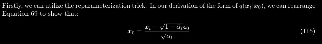
Moving x_{{0}} to the left-hand-side, we get

x_{0} = \frac{x_{{t}}}{\sqrt{\bar{\alpha_{t}}}} - \sqrt{\frac{1- \bar{\alpha_{t}}}{\bar{\alpha_{t}}}}\epsilon

\sqrt{\frac{1- \bar{\alpha_{t}}}{\bar{\alpha_{t}}}} is the sigmas that @KevinB highlighted in his post, Point 4), where he wrote

*\Sigma = \sqrt{\frac{1 - \alpha\_cumprod}{\alpha\_cumprod}}

and is expresed in code as

sigmas = np.array(((1 - alphas_cumprod) / alphas_cumprod) ** 0.5)

Note that alphas_cumprod (\bar{\alpha}) is a cumulative product \prod_{i=0}^t \alpha_{i} , and as pointed out by @KevinB, involves the multiplication of many terms

np.cumprod([1, 2, 3, 4])
> array([1, 2, 6, 24])

So now, if you run the following code, you can get alphas_cumprod or \bar{\alpha}

beta_start = 0.00085
beta_end = 0.012
betas =  torch.linspace(beta_start**0.5, beta_end**0.5, 1000, dtype=torch.float32) ** 2
alphas = 1.0 - betas
alphas_cumprod = torch.cumprod(alphas, dim=0)

and if you run the following code you get sigmas or \sigma = \sqrt{\frac{1- \bar{\alpha_{t}}}{\bar{\alpha_{t}}}}

sigmas = np.array(((1 - alphas_cumprod) / alphas_cumprod) ** 0.5)
sigmas = np.concatenate([sigmas[::-1], [0.0]]).astype(np.float32)
sigmas = torch.from_numpy(sigmas)
print("Sigma max:", sigmas.max())
> Sigma max: tensor(14.6146)

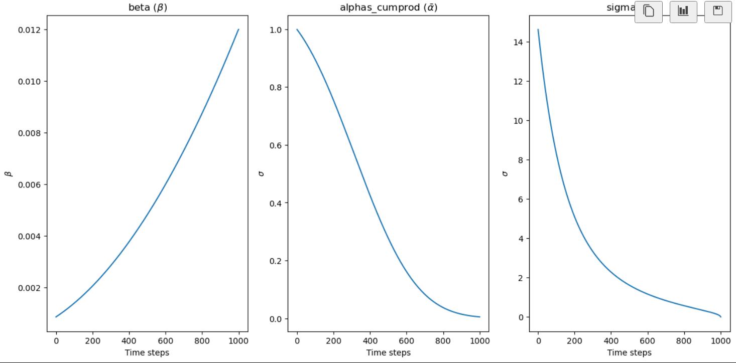
Plot \beta, \sigma and \bar{\alpha} using the following code

fig, axs = plt.subplots(1,3,figsize=(15, 7))

time_step = torch.linspace(0,1000,1000,dtype=torch.int)
axs[0].plot(time_step, betas)
axs[0].set(xlabel = "Time steps", ylabel ="$\\beta$")
axs[0].set_title("beta ($\\beta$)")

time_step = torch.linspace(0,1000,1000,dtype=torch.int)
axs[1].plot(time_step, alphas_cumprod)
axs[1].set(xlabel = "Time steps", ylabel ="$\\sigma$")
axs[1].set_title("alphas_cumprod ($\\bar{\\alpha}$)")

time_step = torch.linspace(0,1001,1001,dtype=torch.int)
time_step = torch.linspace(0,1001,1001,dtype=torch.int)
axs[2].plot(time_step, sigmas)
axs[2].set(xlabel = "Time steps", ylabel ="$\\sigma$")
axs[2].set_title("sigma ($\\sigma$)")

Note that for \beta, instead of a straight-line schedule using

beta = torch.linspace(beta_start, beta_end, noise_steps)

a slighly curved schedule is used for stability diffusion instead

beta =  torch.linspace(beta_start**0.5, beta_end**0.5, 1000) ** 2

---

Tedious Math

The tedious maths to get alpha_cumprod (\bar{\alpha}) is provided below

Source: Understanding Diffusion Models: A Unified Perspective

---