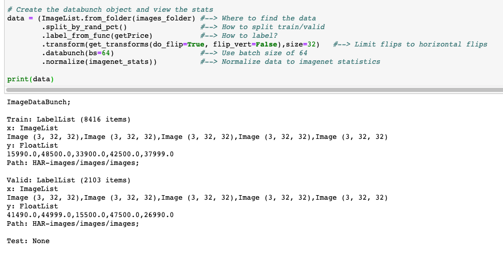
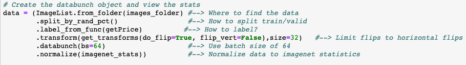
Hello all. I’ve only made it through lesson 3 so far, so feel free to ignore me if this is covered in future lectures. I have approx 10,000 images of houses and their listing prices. Just for fun, my goal is to create an image regression model starting from resnet34 (similar to lectures but not using binary/multi-label classification). I’ve succeeded in building the learner but have run into a problem…
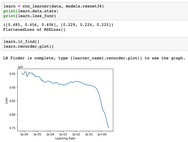
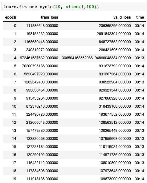
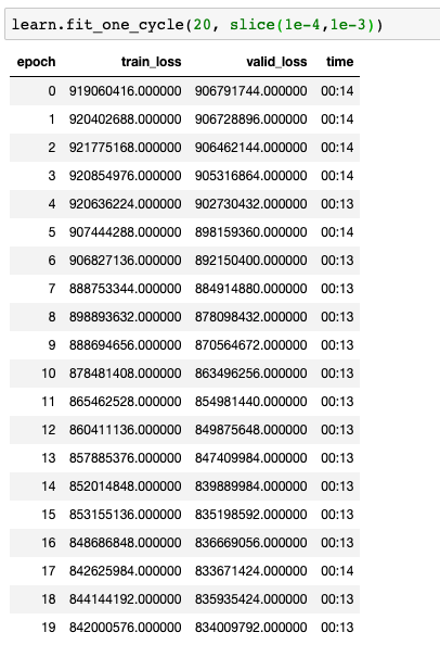
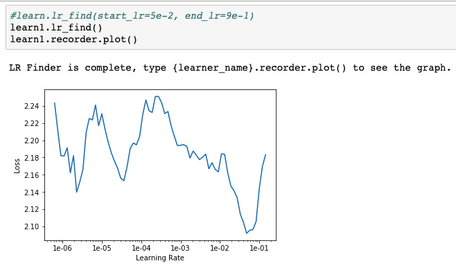
Unfortunately, I have extremely high training and validation loss (massive under-fitting?). I’m using lr_find() to capture a learning rate slice like in lectures, but the method provides a pretty big learning rate for my problem. I first tried 1-10 and then 1-100. Both provide pretty large values for training and validation loss. I’ve used .normalize(imagenet_stats) to normalize my data to the resnet34 model and verified the learner is using MSE for the loss function. I’m not sure what I’m missing but I have a feeling it’s something very fundamental and simple. See snips below…
Don’t forget that your loss is taking the square of the difference between your expected and your predicted prices, and as you are playing with numbers in the order of 1e5, it is completely normal to have such high numbers.
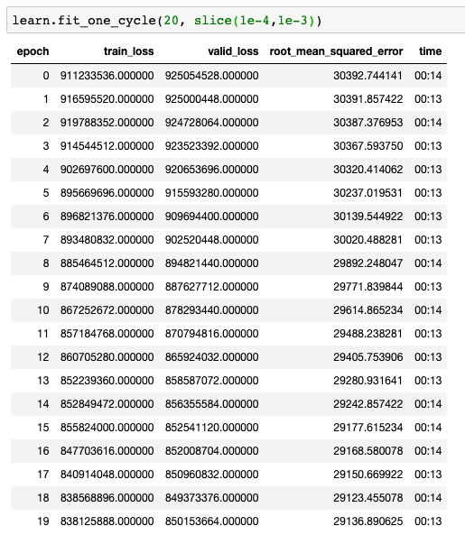
As long as the validation loss is decreasing (it is your case), it means that your model is learning something usefull. Maybe add a metrics = 'root_mean_squared_error' when creating your learner if you want more readable values to assess how your model is doing.
I would just double check your choice of learning rate. In your case, a lr=1 seems enough (look at the instable behaviour that happens at epoch 1 and 4).
Ahhh. This is definitely a fundamental thing I need to dig into and understand.
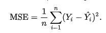
So if the MSE equation is…
Then i’m guessing ‘metrics=root_mean_squared_error’ simply square roots the MSE value. It therefore represents the average error (difference between predicted and actual listing value) over the entire training set, and for that particular epoch (set of weights)?
In other words, the algorithm’s guesses after 1 epoch below would be, on average over the training set, $30,000 off (or really $300,000 since my floating point somehow got screwed up on my labels).
So in my first training slice(1,100), I absolutely see the instability you reference. However, can you explain to me how you deduced from this that “lr = 1 seems enough.” Is that just an educated guess or are you pulling that out of an understanding of precisely how the fit_one_cycle () is distributing the change in learning rate from 1 epoch to another?
Well, this is my first go at building a model of any kind, so I was trying to replicate the lecture flow. Basically, build a model that can perform halfway decent at 32x32 and it should perform better when you use transfer learning to scale up to 64x64. But like I said, I’m just understanding the ropes here, so all advice is welcome.
As you can see, I used mixup. This helps dealing with overfitting
I used smoothed L1 loss. MSE and L1 loss have certain disadvantages and smooth L1 loss takes care of these disadvantages.
Then in last, I used Progressive Image Resizing in which you train on smaller image size, then save the model weights and retrain on higher image sizes
Hope this helps. Let me know if you want to discuss it further
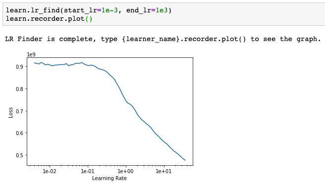
Also, regarding the lr_find, you want to get a value for the lr where the slope is the steepest, so for me your lr should be in the order of 1e0, but definetely not in the order of 1e2. Also, now that you know the order of magnitude your lr will be, you could also probably get a better graph by setting a parameter start_lr and end_lr in your lr_find function, for example:
learn.lr_find(start_lr=1e-3, end_lr=1e3)
It should give you the usual shape as in the Lessons
I really appreciate you taking the time to make the list. I’m going to revisit your list when I make it further in the lectures. The things you’ve mentioned here are taking advantage of some more custom aspects of the library. I need to get my feet under me with the vanilla stuff first
With that said, give me a couple weeks and I know revisiting your list will be very valuable. I’ll let you know when I have questions!
This is probably just due to the scale of the housing prices. You should normalize price data (subtract the mean, divide by the standard deviation), take the log of the data, or both.
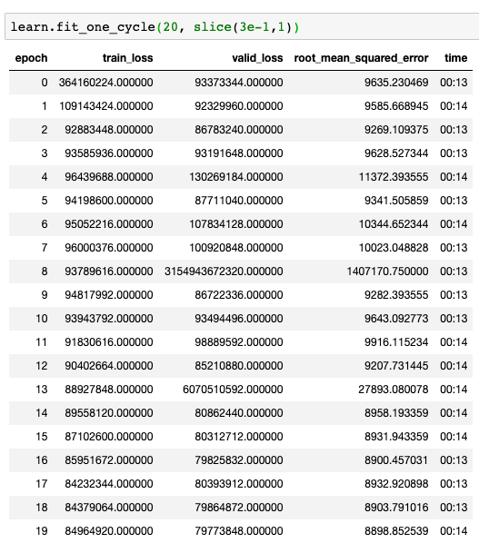
Brilliant Feature and great tip! Looks like slice(3e-1,1) is a good estimate to the steepest slope…
However, still seems unstable. I don’t really have a benchmark for number of epochs though, so maybe the model just needs a lot more time?
Also, maybe @KarlH is correct. I believe normalizing my labels would force the model to calculate smaller weights. I think I’ve read that this can potentially lead to a more stable model, but I’m unsure about the underlying reasoning.
How do I find what activation function is used? Am I saturating the activation functions by using such high value labels? Do I not know what I’m talking about?
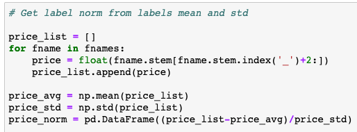
Thanks for the tip!. I’ll have to try this. I’m guessing fast.ai has a builtin databunch method to normalize the labels, but I haven’t found it yet. I can always create a list from the filenames and do the operation myself I suppose…
Do you have any wisdom into if normalizing the labels will actually create a better model (or allow faster training), or will this simply make the loss/error values more intuitive?
Neural networks are pretty finicky about the scale of numbers, because you have lots of operations compounding on each other. If your numbers are too small, they go to zero. If your numbers are too big, they go to infinity.
Because of this, networks tend to be carefully initialized to values that are small but not too small. You’re coming in with these massive output values (real home prices), and asking the network to produce those from small weights. This puts a lot of stress on the network to make that scaling happen, which can lead to poor training or numerical instability. Large values at the end of the network can also be backpropagated into the earlier layers of the network, causing large weight changes which can be detrimental.
This is why in general you want to normalize your inputs and outputs (ie normalizing images by channel, etc). I think you’ll find methods for normalizing structured data in the tabular section of the library, but it’s easy enough to do manually.
Take the log of all home prices (not technically part of normalization, but it helps a lot with dealing with the scale of data, especially if the the values range over different orders of magnitude)
Find the mean and standard deviation of the data
Create normalized values by subtracting the mean and dividing by the standard deviation (X_{norm} = \frac{X - \mu}{\sigma})
Then for training the model you have some options for how you generate your output. The simplest way would be to take the raw logit value out of the network and use that as your output. This should work fine.
Another way is to put your network’s output through a scaled sigmoid function to squash the values to be between the minimum and maximum home prices in the dataset. Look at how this is done in the TabularModel class. I would try both approaches.
Thanks Karl. That jives well, I appreciate the explanation. I’m running into an issue trying to normalize things myself. I’m not sure how to efficiently get it to work with the fastAI library.
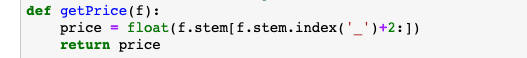
Basically, my data is is just 10,000 images with filenames like 1_390000.png. The first number is just a random index and the second number is the list price.
My idea to normalize was just to take all my labels, normalize them, then throw them into a list… which this does.
However, there is no .labels_from_list() dataBunch method. I tried converting my list to a pandas dataframe, but this didn’t work because .label_from_df() doesn’t accept any sort of dataframe object.
Trying to piece how this works, it seems like label_from_df only if I use the .from_df() method instead of the from_folder() method. This means I need to first preprocess all my image paths and labels into a pandas dataframe like described here…
Good news! I was able to load normalized labels(with corresponding image paths) into a df and build a working dataBunch object and learner.
However, I do not have normalized image channels yet. Still working out how to do this…
My strategy for running the model is as follows:
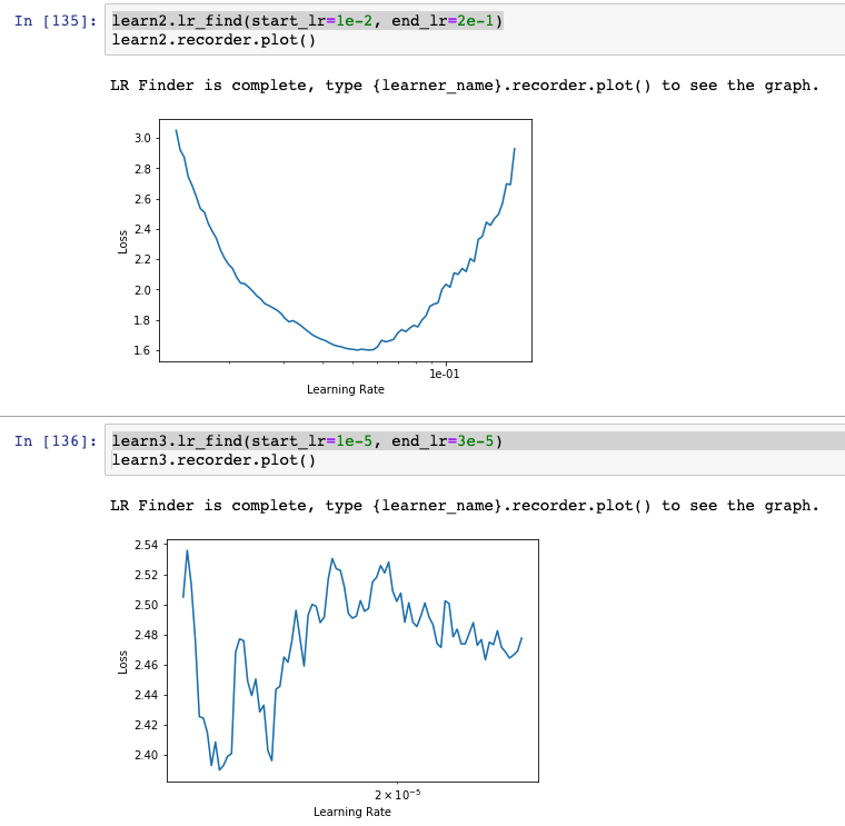
Build a learner and show it’s plot
Find three ranges that look like good candidates for “steepest” slope
Zoom into these ranges using something like `learn3.lr_find(start_lr=1e-5, end_lr=3e-5)’
Study these zoomed-in graphs and choose the best learning rate range I can find.
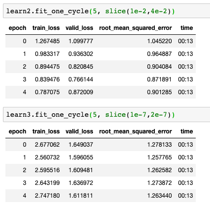
.fit_one_cycle() each of these ranges for 5 epochs and look for the best candidate to continue running for additional epochs (best candidate will be learner where training loss is lowest and decreasing).
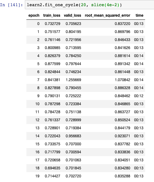
Choose best candidate and run for as many epochs as needed to get a good root_mean_squared_error.
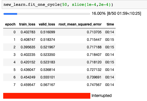
Although there’s definitely improvement here… I’m still fighting to get training loss lower than the validation loss (and for a constantly decreasing error). I can run for more epochs, but I feel like my learning rate is still off. Any thoughts? Below are the results.
As can be seen, training loss is jumping around a bit but, on the whole, decreasing. However, training loss is still above validation loss, so still under-fitting. I can run for more epochs but don’t really have a good feel for the “speed” the network should be learning (if i’m in the right learning rate ballpark). I’m not sure whether I should spend time trying to figure out how to normalize the image channels or train for more epochs. Thoughts?
You don’t have to worry about normalizing the input image. That’s done when you add .normalize(imagenet_stats) to your data.
Are you unfreezing the model? I don’t see that in any of the images you posted. If not you should definitely do that. Without unfreezing you’re only training the linear head of the model, not the entire model.
And that’s correct, I hadn’t yet unfreezed the model. After you mentioned this, however… I did unfreeze and ran a few experiments. Unfortunately, I think I ran into overfitting after running ±250 epochs. I think I might start fresh and try to find a higher learning rate that works or bump the images up to 64x64. If this doesn’t work I guess I’ll have to dig a little deeper into network architectures and the list from @abhikjha. I haven’t yet reached a lecture that discusses overfitting in detail, but I’m guessing that will come later in the course.
Is there a good rule of thumb on when is an appropriate time to unfreeze? After seeing a certain loss value? After a certain number of epochs with continual loss decrease? etc?