How does back-prop factor in the changes that the rest of the network is going to make in weight updates?

Or to rephrase the same idea (I think) - if a network is only being trained on one example; and a small enough learning rate is being used; can back-prop guarantee to always reduce the cost function?

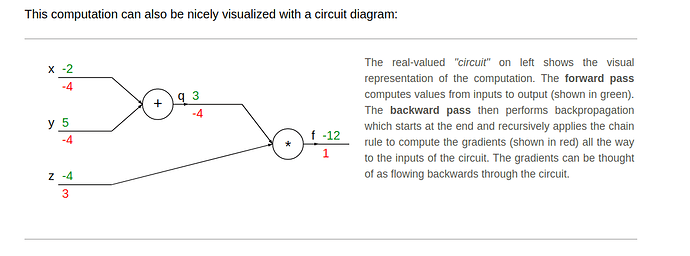
From https://cs231n.github.io/optimization-2/ there is the below screen shot.

Since y & z have different gradients; they are going to get “opposite” deltas depending in which direction f’s output is desired to go. However; if z’s delta ends up in changing z’s sign; then that means y’s delta becomes in the “wrong” direction. With the values given in the example; a small learning rate would make sure z’s sign doesn’t change; but once z was close to 0; it seems the scenario of z’s sign change making y’s delta be the wrong direction would occur.

Does the “full” back-prop algorithm have a way of handling this? As I (very partially) understand; back-prop only requires one forward propagation pass; so I don’t think it’s a case of updating a weight; and then calculating derivatives based off the value of the new weight.

Hi Brent. It took a whole round of brushing my teeth to understand your confusion.

I think you are bothered by the possibility that updating weight z alone might change the sign of y’s gradient at the partially updated weight vector.

The short answer is - it doesn’t matter. Once the other weights are updated, the loss will go down. SGD claims nothing about the gradient for the fully or partially updated weights, and does not need to in order to work. It only needs the loss to go down. What happens with steps along the axes is irrelevant.

The simplest way to think of this is as a multidimensional calculus situation. A basic theorem is that if you take a small enough step in the negative direction of the gradient, the function will decrease (given some conditions on the weights->loss function).

HTH, Malcolm

Hi Malcolm; thank you for dedicating a portion of your days brain capacity to my somewhat unclear question, much appreciated! As I’m reading your answer; it occurred to me that the “small enough step” aspect would be relevant even if only updating a single weight at a time.

And; I did want to confirm that there was not an “update single weight; then calculate rest of weight updates with this new weight” part of the algorithm, so thanks.

Glad my brain capacity could clarify something today.

Now, why isn’t my model training? :confused:

This is clawing at the limit of my understanding, but:

The gradient is made up of partial derivatives, i.e. dL/dy assumes x and z are not changing. So changing y based on its partial derivative does not take into account that we’re also going to be changing x and z based on their own derivatives.

However, since dL/dy tells us what we need to do to y to lower the loss, and dL/dx and dL/dz tell us what we need to do to x and z to lower the loss, you can assume that the loss is indeed going down on average.

I guess it can happen that changing both y and z will actually make the loss larger because of the interplay between those variables (i.e. we’re not actually holding z constant even though dL/dy assumes we do) but my math-fu isn’t strong enough to prove or disprove this.

1 Like

Hi again. I created some confusion with my first reply, and would like to clear it up. Hopefully without adding more confusion!

The theorem from calculus is right in theory, but not very relevant in practice. It lets us be confident that gradient descent methods will lead to a local minimum if the step is small enough. But once momentum and fancy optimizers come into the picture, all bets are off. These try to estimate a step that makes the loss decrease the most. That step could be many times larger than the calculus step, not exactly in the gradient direction, and may even be wrong. In fact, the loss occasionally increases after a weight update. (Note that fastai’s loss graph display is smoothed, so you don’t see many loss increases.)

Sorry for my misleading theoretical answer. Brent @bgraysea you are right that the update is done all at once. The only new information that the optimizer has to work with at the update is the current weights and the current gradient. It may also have saved running averages of these (momentum, Adam), or the previous gradients (2nd order optimizer). It then uses everything to come up with a direction and size for the “best” step. But the outcome is not guaranteed by theory.

Here’s some musings, and all that follows are just my opinions. The Universal Approximation Theorem say that if a model is complex enough then it can approximate any function. But no one would ever use its construction in practice. The model it gives would have an enormous number of units, and who knows if it would even generalize to new data. Instead we use working, practical knowledge of which architectures work well in which domains. These models fit in a GPU, train well, and generalize. Still, the UAT gives us confidence that what we are trying to achieve is possible, not futile.

Likewise, the calculus theorem tells us that gradient descent methods, in general, work. But no one would train with tiny steps in the negative gradient direction. We now have practical knowledge about optimizers that take bigger steps approximately along the gradient, and train faster overall. Still, calculus theorems tells us that this is a reasonable approach.

Matt @machinethink, if you will forgive me for any misunderstandings, I think your scenario applies to a large step size. The loss can indeed go up, as you point out. Way “out there” from the current weights there are no guarantees about the loss value or its gradients. But if you make the step size smaller and smaller there will come a step size where the loss is guaranteed to decrease.

Thanks for reading my post and for the chance to clarify!
1 Like

Just to add on one more small thing: it’s OK that optimizers with momentum don’t really follow the gradients (like @Pomo explained). The gradients are already an approximation anyway (and a very rough one at that), because we only look at a small mini-batch instead of the entire training set.

Instead of a single loss function we have N different loss functions where N is the number of mini-batches. So in each iteration we’re actually stepping through the landscape of a totally different loss function.

Thanks for all the great points!!!