I read the Transformer/Attention Is All You Need paper recently, and I thought their “scaled dot-product attention” mechanism was a really nice, memorable example of some of the different ways to think about matrix multiplication, and that it might be useful to walk through:

(I’m going to ignore the \sqrt{d_k} scaling part since it’s not so interesting from a matrix-algebra perspective.)
For a little background, the general idea of attention is to crunch n things down to 1 thing by taking a weighted combination (in particular, one where the weights are all non-negative and sum to 1—a convex combination). For example, the paper Neural Machine Translation by Jointly Learning to Align and Translate proposes a simple seq2seq translation model that uses attention. The encoder provides the n things, an “annotation” vector for each input token, and at each decoding step the decoder crunches them down to 1 thing: it uses whatever it’s currently in the middle of doing to inform how to attend to/convex-ly crunch all those n annotations down to a single vector, tailored to the current decoding step, which then gets fed into the rest of the decocoding machinery.
Anyways, about the Transformer’s attention blocks. Each block takes n input vectors (whatever they may be at that point in the architecture) and produces n output vectors. Attention is apparently all you need, so each output is gonna be some convex combination of… something, some other vectors. The paper calls them “values”. They’re the rows of V in the equation above. They’re some learned function of the inputs—the paper proposes basically the simplest option, a matrix multiplication of the inputs (a Linear layer, if you prefer). [Actually, I’m a little fuzzy on what the paper says to do get the Q, K, and V matrices, but e.g. AllenNLP does seem to use a learned matrix multiply of the input—let me know if I’ve misunderstood this part.]
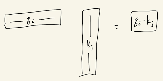
What about the weights of all these convex combinations we need to do? The paper proposes another simple approach: map each input vector to two new vectors, a “query” q and a “key” k, and use them to get a measure of how relevant the j-th input is to the i-th output: just take the dot product of q_i with k_j. In matrix language, this is q k^T:

We can compute all of these dot product relevancy scores for the i-th input “in parallel” by stacking all of the keys into a big matrix (K^T above) and letting matrix multiplication do its thing:
To convert these scores (which could be arbitrary, negative, etc.) into convex weights (non-negative and sum to one), we use our old friend, softmax.
We want to compute these scores not just for the i-th input, but for all the inputs. We can again do everything in parallel with matrix multiplication:

This is Q K^T in the equation above. The softmax to convert from scores to weights happens independently over each row of the output, so that the i-th row of softmax(QK^T) is a vector of weights (non-negative, sum to one).
Ok, now we want to finally take weighted linear combinations of the values (the V in the equation above). The matrix math we’ve used so far is based on what you might call the “dot-product interpretation” of matrix multiplication: you’re dot-ing every row of the matrix on the left with every column of the matrix on the right, “in parallel”, so to speak, and collecting all the results in another matrix. But there’s another equivalent-but-quite-different way to think of matrix multiplication: each row of the matrix on the left is a vector of weights for taking a linear combination of the rows of the matrix on the right! Gilbert Strang calls this the “row interpretation”; there’s also the “column interpretation”, where the columns of the matrix on the right are weights for taking linear combinations of the columns of the matrix on the left. And as usual, this all happens “in parallel”: in the column-interpretation, each column on the right produces its own linear combination of the columns of the matrix on the left, and they all get stacked together column-by-column in the output matrix; and in the row-interpretation, each row on the left produces its own linear combination of the rows of the matrix on the right, and they all get stacked together row-by-row in the output matrix.

So, softmax(Q K^T) produces n rows of weights, and multiplying it on the right by the values V does just what we want: by the row-interpretation, the i-th row of softmax(QK^T)V is a linear combination of the rows of V (what we’re trying to do) according to the weights from the i-th row of softmax(QK^T).
Anyways, hopefully this was fun to work through!

