Forum Markdown Notes - Lesson 8

[timlee]

Hi All,

There’s plenty of other notes out there for lesson 8. I thought I would put a forum version, incase thats useful for others instead of jumping to an external github. Hope its helpful!

If there’s a better place for notes, or contributions, happy to move this post as well

Can always clone if needed: https://github.com/timdavidlee/fastai_dl2019p2

Best,

Tim

Lesson 8 Introduction

Welcome to the course, for those of you who come every year, its a very different course.

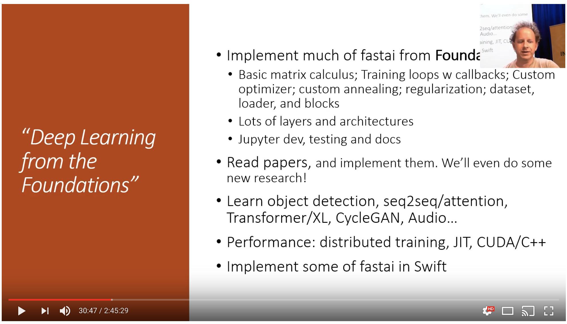
What we will do

• Implement fastai library from foundations (from scratch).

• Read and implement papers

• Implementing much of pytorch

• Going deeper into applications that are not fully-baked in yet

• seq2seq

• attention

• Transformer

• Use JIT / CUDA

• Last 2 lessons, implementing some lessons in Swift

• Part 1 was more practical, learn a technique and use it

• So whats this classes approach? We will teach you the tools to implement papers, experiment with them, and try them out for yourselves

• We used to call part 2 cutting edge, but now the cutting edge is now the engineering part of deep learning. The most effective people are the ones who can successfully build and deploy models

• Part 1 was topdown, saw how deep learning is used in practice, and how to use it, and how to get results

• Part 2 will be bottom up: lets you see the connections between the various things. then you can customize your algo for your own problem, doing the things you need it to do.

• Chris Lattner: build LLVM, built the default compiler C++ clang. And he built Swift, and is now focusing on deep learning

• None of the previous languages were designed for the multi-processor operations, designed by a compiler specialists

• Another option is Julia for numerical programming, which is farther along; So now there are two choices.

• (Jeremy) played around with the swift library over the xmas break.

S4TF = swift for tensoflow

Implement Fastai and Pytorch functionality

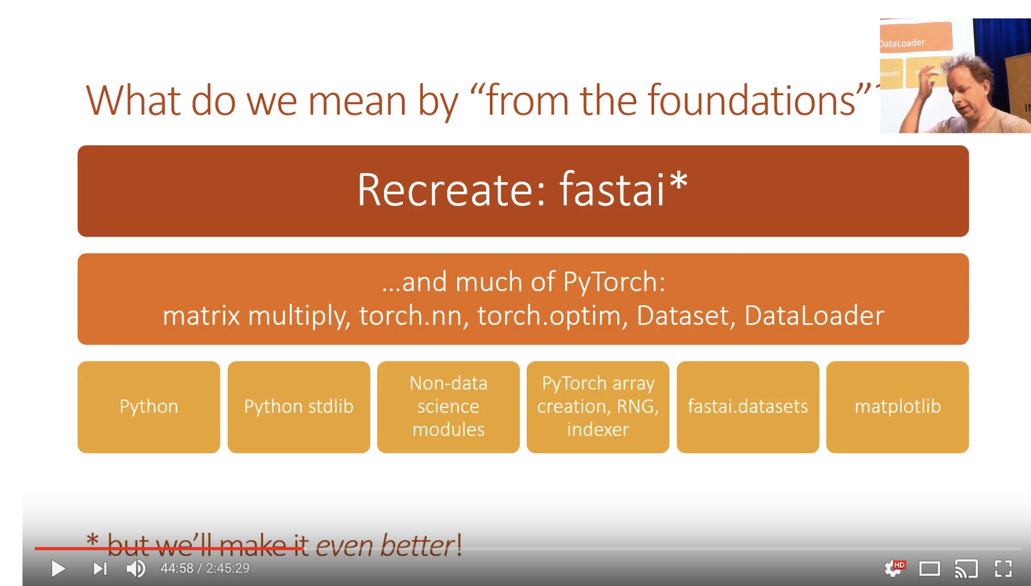
Rules

• We are allowed to use pure python

• Standard python library

• Non-data sci modules

• pytorch - only for arrays and rng

• fastai.datasets (for source materials)

• matplotlib

• Once we recreate a function we can use the real version downstream

Intention

From part 1

For topics that you don’t master, go back to the previous lesson.

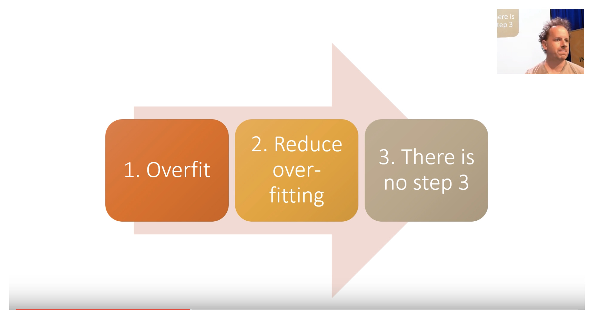
Train really good models.

1. overfit (make sure you have too much predictive power)

2. Reduce the overfitting

3. [there is no step 3] Understand the model

How to reduce overfitting

• This should be the order in while you deal and reduce overfitting

• Many beginner students go in reverse and try to limit architecture complexity, which should be the last thing to be done

Read papers

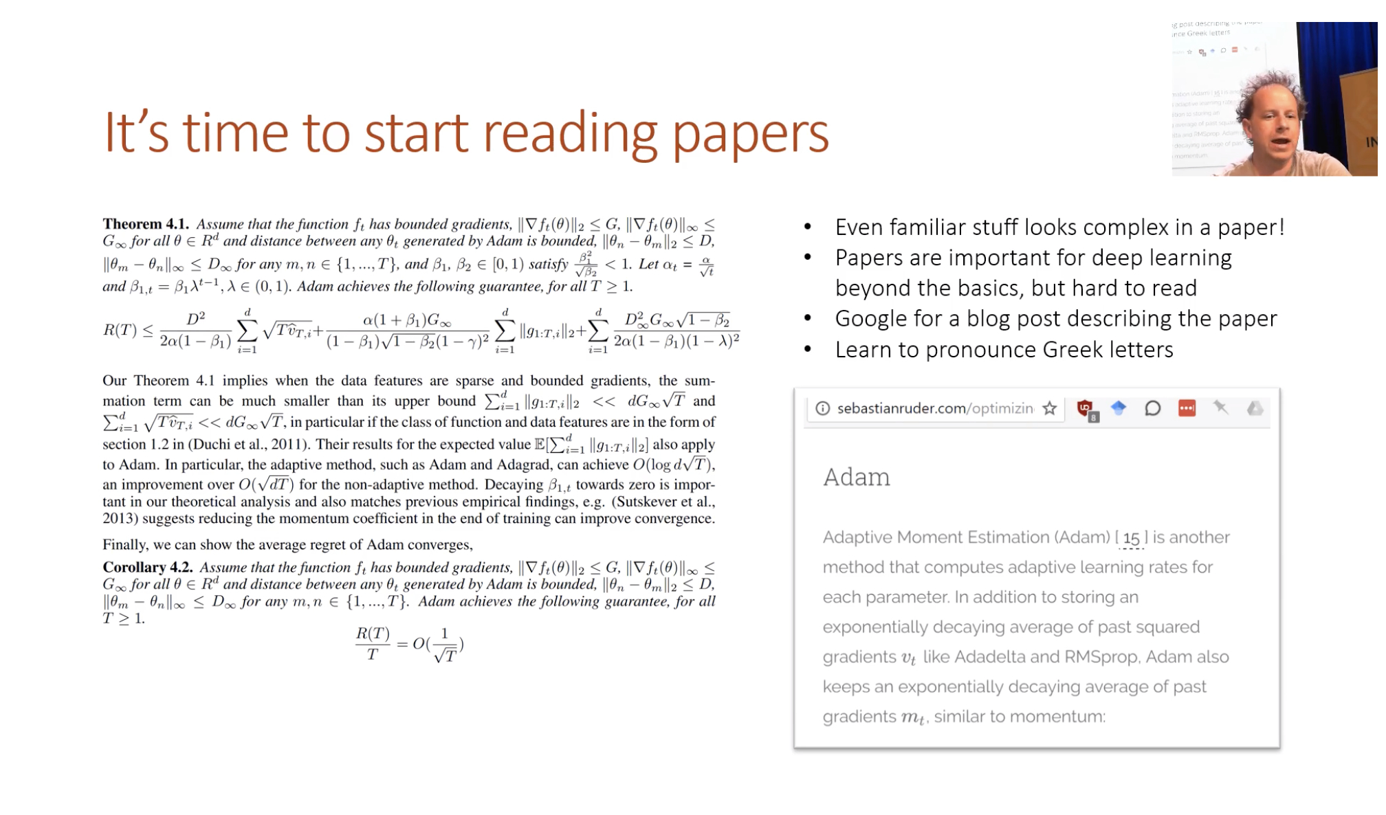
Papers can be very intimidating to read. The simplest of calculations on excel can be a large jumble of symbols in a paper.

Tip 1: learn to pronounce the greek letters, makes equations more approachable.

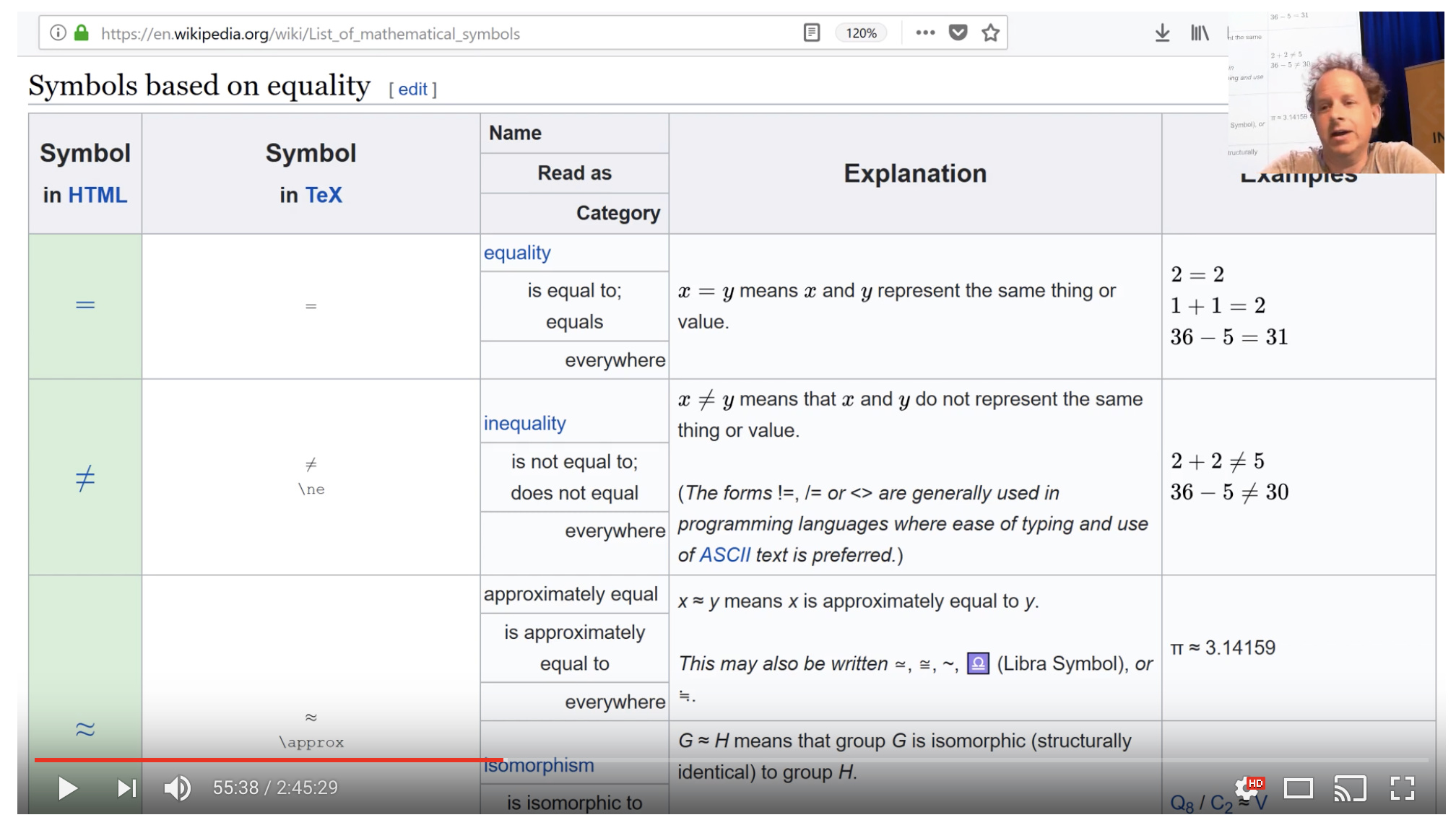
Tip 2: Learn the math symbols - check wikipedia. Detexify - uses machine learning to determine what symbols you are looking at. The nice thing about this is it gives the latex.

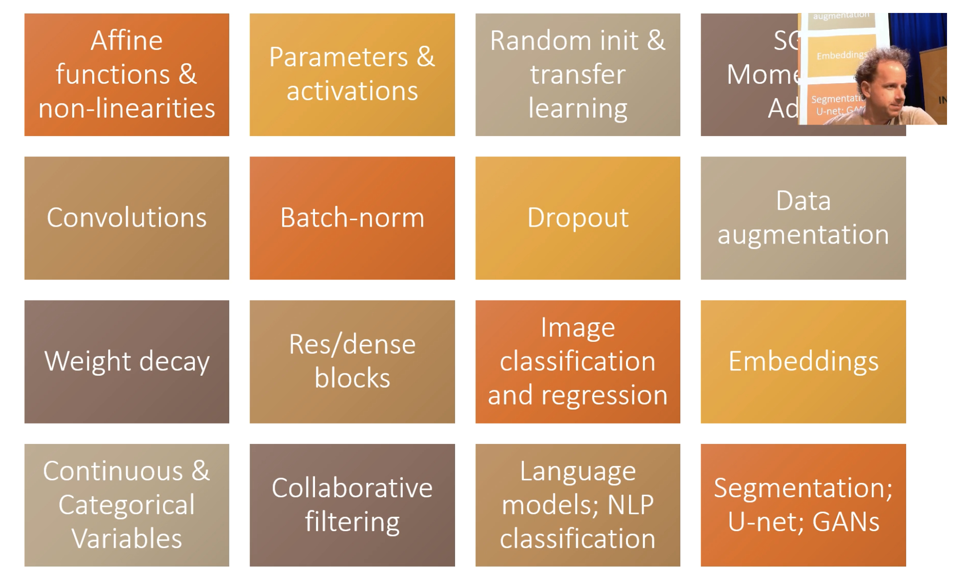
Course Overview

For the next few lessons. We will be making a competant CNN model.

Fastai 2019: Lesson 8.1 - Dev Setup

Lessons can be found : https://github.com/fastai/fastai_docs/tree/master/dev_course/dl2

Covering:

• https://github.com/fastai/fastai_docs/blob/master/dev_course/dl2/00_exports.ipynb

These notes will try and follow the lesson as close as possible, without jumping around to too many files. For this particular course, the libraries being built will be done via Notebooks, instead of the traditional .py files. There’s currently a helper file in this directory called notebook2script.py that will convert cells into functions

Sample export cell

Prerequistes: pip install fire

mkdir exp

What to run:

$python notebook2script.py 00_exports.ipynb

This will go through a particular notebook, and will find the cells with #exports

#export
TEST = 'test'

!mkdir exp

mkdir: exp: File exists

!python notebook2script.py lesson81.ipynb

Converted lesson81.ipynb to nb_lesson81.py

Load the saved constant

Now that the above should have been created, we should be able to import the variable TEST. For the purpose of notes, the functions will be written in a longer format instead of the compact version found in the lesson

from exp.nb_lesson8 import *
import operator


def test(a, b, cmp, cname=None):
    """
    Simple test function
    """
    # if no name is passed, 
    if cname is None: 
        cname=cmp.__name__

    # this is the test
    # if it fails, the second phrase will be returned
    # which is the f"{cname}:\n{a}\n{b}"
    assert cmp(a, b), f"{cname}:\n{a}\n{b}"

def test_eq(a,b):
    """
    Is a larger function that calls the test function
    but only passes teh == sign
    """
    test(a, b, operator.eq, '==')

Run a sample test

If correct, you won’t get any feedback

test_eq(TEST, "test")

If it was wrong you should get a message as follows:

test_eq(TEST, "nottest")

    -
    AssertionErrorTraceback (most recent call last)
    <ipython-input-5-24a85abd2d33> in <module>
    ----> 1 test_eq(TEST, "nottest")

    <ipython-input-3-82ec92dcee6d> in test_eq(a, b)
         21     but only passes teh == sign
         22     """
    ---> 23     test(a, b, operator.eq, '==')

    <ipython-input-3-82ec92dcee6d> in test(a, b, cmp, cname)
         14     # if it fails, the second phrase will be returned
         15     # which is the f"{cname}:\n{a}\n{b}"
    ---> 16     assert cmp(a, b), f"{cname}:\n{a}\n{b}"
         17 
         18 def test_eq(a,b):

    AssertionError: ==:
    test
    nottest

test_eq(TEST, "test")

How to run tests outside the notebook

run_notebook.py will do this

python run_notebook.py lesson8.ipynb

What’s in run_notebook.py

#!/usr/bin/env python

import nbformat,fire
from nbconvert.preprocessors import ExecutePreprocessor

def run_notebook(path):
    nb = nbformat.read(open(path), as_version=nbformat.NO_CONVERT)
    ExecutePreprocessor(timeout=600).preprocess(nb, {})
    print('done')

if __name__ == '__main__': fire.Fire(run_notebook)

• nbformat lets you run a notebook and print out any errors
• fire takes any function and turns it into a command line interface, this manages arguments and other input values

Example

! python run_notebook.py

Will return the function inputs / parameters

    Fire trace:
    1. Initial component
    2. ('The function received no value for the required argument:', 'path')

    Type:        function
    String form: <function run_notebook at 0x102a03f28>
    File:        ~/myrepos/fastai_dl2019p2/live_notes/run_notebook.py
    Line:        6

    Usage:       run_notebook.py PATH
                 run_notebook.py --path PATH

What’s in notebook2script.py

#!/usr/bin/env python

import json,fire,re
from pathlib import Path

def is_export(cell):
    if cell['cell_type'] != 'code': return False
    src = cell['source']
    if len(src) == 0 or len(src[0]) < 7: return False
    #import pdb; pdb.set_trace()
    return re.match(r'^\s*#\s*export\s*$', src[0], re.IGNORECASE) is not None

def notebook2script(fname):
    fname = Path(fname)
    fname_out = f'nb_{fname.stem.split("_")[0]}.py'
    main_dic = json.load(open(fname,'r'))
    code_cells = [c for c in main_dic['cells'] if is_export(c)]
    module = f'''
#################################################
### THIS FILE WAS AUTOGENERATED! DO NOT EDIT! ###
#################################################
# file to edit: dev_nb/{fname.name}
'''
    for cell in code_cells: module += ''.join(cell['source'][1:]) + '\n\n'
    # remove trailing spaces
    module = re.sub(r' +$', '', module, flags=re.MULTILINE)
    open(fname.parent/'exp'/fname_out,'w').write(module[:-2])
    print(f"Converted {fname} to {fname_out}")

if __name__ == '__main__': fire.Fire(notebook2script)

One of the key observations is that notebooks are json. Hence the line:

main_dic = json.load(open(fname,'r'))

For example, loading this lesson notebook can be done by the following:

import json
notebook_as_json_cells = json.load(open("lesson8.ipynb","r"))["cells"]
notebook_as_json_cells[2]

{'cell_type': 'code',
 'execution_count': None,
 'metadata': {},
 'outputs': [],
 'source': ['#export\n', "TEST = 'test'"]}

Fastai 2019: Lesson 8 - Matrix Multipication

First we will do some basic imports. The following notebook magic lines will do the following

• will auto reload external references or files
• and will do so on a specific interval
• will plot in the notebook
• matplotlib mpl will use gray scale since we are going to be working with MNIST

%load_ext autoreload
%autoreload 2

%matplotlib inline
mpl.rcParams['image.cmap'] = 'gray'

import operator


def test(a, b, cmp, cname=None):
    """
    Simple test function
    """
    # if no name is passed, 
    if cname is None: 
        cname=cmp.__name__

    # this is the test
    # if it fails, the second phrase will be returned
    # which is the f"{cname}:\n{a}\n{b}"
    assert cmp(a, b), f"{cname}:\n{a}\n{b}"

def test_eq(a,b):
    """
    Is a larger function that calls the test function
    but only passes teh == sign
    """
    test(a, b, operator.eq, '==')

#export

# standard libraries
from pathlib import Path
from IPython.core.debugger import set_trace
import pickle, gzip, math, torch, matplotlib as mpl
import matplotlib.pyplot as plt

# datasets
from fastai import datasets

# basic pytorch
from torch import tensor

MNIST_URL='http://deeplearning.net/data/mnist/mnist.pkl'

Download the mnist dataset and load

path = datasets.download_data(MNIST_URL, ext='.gz'); path

# unzips the download
with gzip.open(path, 'rb') as f:
    ((x_train, y_train), (x_valid, y_valid), _) = pickle.load(f, encoding='latin-1')

# maps the pytorch tensor function against each
# of the loaded arrays to make pytorch versions of them
x_train,y_train,x_valid,y_valid = map(tensor, (x_train,y_train,x_valid,y_valid))

# store the number of 
# n = rows
# c = columns
n,c = x_train.shape

# take a look at the values and the shapes
x_train, x_train.shape, y_train, y_train.shape, y_train.min(), y_train.max()

(tensor([[0., 0., 0.,  ..., 0., 0., 0.],
         [0., 0., 0.,  ..., 0., 0., 0.],
         [0., 0., 0.,  ..., 0., 0., 0.],
         ...,
         [0., 0., 0.,  ..., 0., 0., 0.],
         [0., 0., 0.,  ..., 0., 0., 0.],
         [0., 0., 0.,  ..., 0., 0., 0.]]),
 torch.Size([50000, 784]),
 tensor([5, 0, 4,  ..., 8, 4, 8]),
 torch.Size([50000]),
 tensor(0),
 tensor(9))

Lets test our input data

1. row check: check that the number of rows in x_train is teh same shape as y_train and that number should be 50,000
2. column check: check that number of columns is 28*28 because that is the total number of pixels of the unrolled images
3. classes check: test that there are 10 different classes found in y_train: 0 - 9

assert n==y_train.shape[0]==50000
test_eq(c,28*28)
test_eq(y_train.min(),0)
test_eq(y_train.max(),9)

Take a peek at one of the images

img = x_train[0]
img.view(28,28).type()

'torch.FloatTensor'

# note that there is a single vector that is reshaped into the square format
plt.imshow(img.view((28,28)));

Initial Model

We will first try and linear model:

A = wx + b will be the first model that we will try. We will need the following:

• w: weights
• b: baseline or bias

weights = torch.randn(784,10)
bias = torch.zeros(10)

Matrix Multiplication

We will be doing this alot, so its good to get familiar with this. There’s a great website called matrixmultiplication.xyz that will illustrate how matrix multiplication works.

Matrix multiplication function

The following function multiplies two arrays element by element

def matmul(a,b):
    
    # gets the shapes of the input arrays
    ar,ac = a.shape # n_rows * n_cols
    br,bc = b.shape
    
    # checks to make sure that the
    # inner dimensions are the same
    assert ac==br
    
    # initializes the new array
    c = torch.zeros(ar, bc)
    
    # loops by row in A
    for i in range(ar):
        
        # loops by col in B
        for j in range(bc):
            
            # for each value
            for k in range(ac): # or br
                c[i,j] += a[i,k] * b[k,j]
    return c

Let’s do a quick sample

Will use the first 5 images from the validation data and multiply them by the weights of the matrix

m1 = x_valid[:5]
m2 = weights
m1.shape, m2.shape

(torch.Size([5, 784]), torch.Size([784, 10]))

will time the operation

%time t1=matmul(m1, m2)

CPU times: user 605 ms, sys: 2.21 ms, total: 607 ms
Wall time: 606 ms

t1.shape

torch.Size([5, 10])

How can we do this faster?

We can do this with element-wise operations. We will use pytorch’s tensor to illustrate this. When using pytorch objects, Operators (+,-,*,/,>,<,==) are usually element-wise. Examples of element-wise operations:

a = tensor([10., 6, -4])
b = tensor([2., 8, 7])
m = tensor([[1., 2, 3], [4,5,6], [7,8,9]]); 
a, b, m

(tensor([10.,  6., -4.]), tensor([2., 8., 7.]), tensor([[1., 2., 3.],
         [4., 5., 6.],
         [7., 8., 9.]]))

# Addition
print(a + b)

# comparisons
print(a < b)

# can summarize
print((a < b).float().mean())

# frobenius norm
print((m*m).sum().sqrt())

tensor([12., 14.,  3.])
tensor([0, 1, 1], dtype=torch.uint8)
tensor(0.6667)
tensor(16.8819)

If we adjust the matmul

for k in range(ac): # or br
    c[i,j] += a[i,k] * b[k,j]

will be replaced by

c[i,j] = (a[i,:] * b[:,j]).sum()

def matmul(a,b):
    
    # gets the shapes of the input arrays
    ar,ac = a.shape # n_rows * n_cols
    br,bc = b.shape
    
    # checks to make sure that the
    # inner dimensions are the same
    assert ac==br
    
    # initializes the new array
    c = torch.zeros(ar, bc)
    
    # loops by row in A
    for i in range(ar):
        
        # loops by col in B
        for j in range(bc):
            
            c[i,j] = (a[i,:] * b[:,j]).sum()
    return c

After the performance changes, the multiplication is much much faster

%time t1=matmul(m1, m2)

CPU times: user 1.57 ms, sys: 864 µs, total: 2.44 ms
Wall time: 1.57 ms

To test it we will write another function to compare matrices. The reason for this is that due to rounding errors from math operations, matrices may not be exactly the same. As a result, we want a function that will “is a equal to b within some tolerance”

#export
def near(a,b): 
    return torch.allclose(a, b, rtol=1e-3, atol=1e-5)

def test_near(a,b): 
    test(a,b,near)

test_near(t1, matmul(m1, m2))

Broadcasting

The term broadcasting describes how arrays with different shapes are treated during arithmetic operations. The term broadcasting was first used by Numpy.

From the Numpy Documentation:

The term broadcasting describes how numpy treats arrays with 
different shapes during arithmetic operations. Subject to certain 
constraints, the smaller array is “broadcast” across the larger 
array so that they have compatible shapes. Broadcasting provides a 
means of vectorizing array operations so that looping occurs in C
instead of Python. It does this without making needless copies of 
data and usually leads to efficient algorithm implementations.

In addition to the efficiency of broadcasting, it allows developers to write less code, which typically leads to fewer errors.

Example: broadcasting against a constant scalar

a

tensor([10.,  6., -4.])

a > 0

tensor([1, 1, 0], dtype=torch.uint8)

a + 1

tensor([11.,  7., -3.])

2 * m

tensor([[ 2.,  4.,  6.],
        [ 8., 10., 12.],
        [14., 16., 18.]])

How are we able to do a > 0? 0 is being broadcast to have the same dimensions as a.

For instance you can normalize our dataset by subtracting the mean (a scalar) from the entire data set (a matrix) and dividing by the standard deviation (another scalar), using broadcasting.

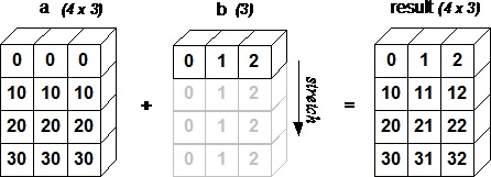
Example: broadcasting vector against a matrix

c = tensor([10.,20,30]); c

tensor([10., 20., 30.])

m

tensor([[1., 2., 3.],
        [4., 5., 6.],
        [7., 8., 9.]])

m.shape,c.shape

(torch.Size([3, 3]), torch.Size([3]))

m + c

tensor([[11., 22., 33.],
        [14., 25., 36.],
        [17., 28., 39.]])

c + m

tensor([[11., 22., 33.],
        [14., 25., 36.],
        [17., 28., 39.]])

We don’t really copy the rows, but it looks as if we did. In fact, the rows are given a stride of 0.

t = c.expand_as(m)
t

tensor([[10., 20., 30.],
        [10., 20., 30.],
        [10., 20., 30.]])

m + t

tensor([[11., 22., 33.],
        [14., 25., 36.],
        [17., 28., 39.]])

# even though it may appear to be a 3x3, if we 
# look at the memory, its only storing a single copy
t.storage()

 10.0
 20.0
 30.0
[torch.FloatStorage of size 3]

# the stride, tells when it is going
# row to row, it takes 0 steps (constant values)
# column to column it takes 1 step
t.stride(), t.shape

((0, 1), torch.Size([3, 3]))

You can index with the special value [None] or use unsqueeze() to convert a 1-dimensional array into a 2-dimensional array (although one of those dimensions has value 1). This will be important later when using matrix multiplication in modeling

print(c.unsqueeze(0))

tensor([[10., 20., 30.]])

print(c.unsqueeze(1))

tensor([[10.],
        [20.],
        [30.]])

m

tensor([[1., 2., 3.],
        [4., 5., 6.],
        [7., 8., 9.]])

c.shape, c.unsqueeze(0).shape,c.unsqueeze(1).shape

(torch.Size([3]), torch.Size([1, 3]), torch.Size([3, 1]))

c.shape, c[None].shape,c[:,None].shape

(torch.Size([3]), torch.Size([1, 3]), torch.Size([3, 1]))

Note the change from a size 3 to a 1 x 3 or a 3 x 1.

The syntax can also be shortened as follows:
You can always skip trailling ':'s. And '...' means ‘all preceding dimensions’

c[None].shape,c[...,None].shape

(torch.Size([1, 3]), torch.Size([3, 1]))

m + c[:,None]

tensor([[11., 12., 13.],
        [24., 25., 26.],
        [37., 38., 39.]])

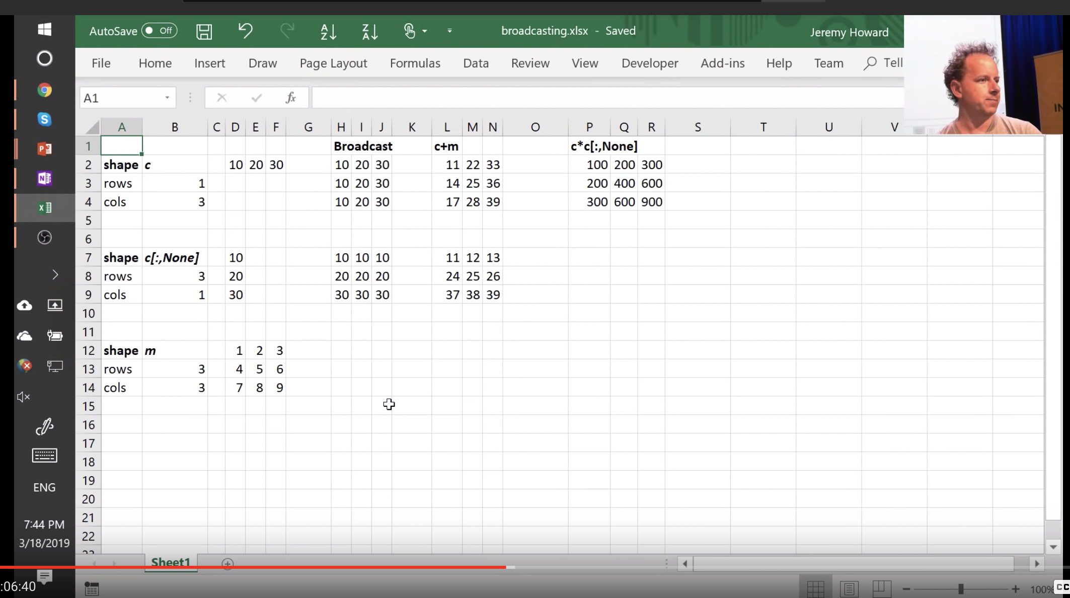
Excel can be very helpful

Here is an excel sheet illustrating broadcasting

Back to our function

Lets take advantage of broadcasting and reduce the loops in our matmul function:

We will replace:

    # loops  by col in B
        for j in range(bc):
            
            c[i,j] = (a[i,:] * b[:,j]).sum()

With

c[i] = (a[i].unsqueeze(-1) * b).sum(dim=0)

So what’s happening

a[i,:] looks at a rank 1 tensor

.unsqueeze(-1) makes it 2d, the -1 means the last dimension

* b broadcast over b

.sum(dim=0) sum along the first axis

def matmul(a,b):
    
    # gets the shapes of the input arrays
    ar,ac = a.shape # n_rows * n_cols
    br,bc = b.shape
    
    # checks to make sure that the
    # inner dimensions are the same
    assert ac==br
    
    # initializes the new array
    c = torch.zeros(ar, bc)
    
    # loops by row in A
    for i in range(ar):
        c[i] = (a[i].unsqueeze(-1) * b).sum(dim=0)
    return c

%time t1=matmul(m1, m2)

CPU times: user 440 µs, sys: 283 µs, total: 723 µs
Wall time: 421 µs

test_near(t1, matmul(m1, m2))

Broadcasting Rules

Since multi-dimensional broadcasting can be complicated, make sure to follow some of the rules

When operating on two arrays/tensors, Numpy/PyTorch compares their shapes element-wise. It starts with the trailing dimensions, and works its way forward. Two dimensions are compatible when

• they are equal, or
• one of them is 1, in which case that dimension is broadcasted to make it the same size

Arrays do not need to have the same number of dimensions. For example, if you have a 2562563 array of RGB values, and you want to scale each color in the image by a different value, you can multiply the image by a one-dimensional array with 3 values. Lining up the sizes of the trailing axes of these arrays according to the broadcast rules, shows that they are compatible:

    Image  (3d array): 256 x 256 x 3
    Scale  (1d array):             3
    Result (3d array): 256 x 256 x 3

Consider the following examples

# add column in front
c[None,:]

tensor([[10., 20., 30.]])

c[None,:].shape

torch.Size([1, 3])

# add column in back
c[:,None]

tensor([[10.],
        [20.],
        [30.]])

c[:,None].shape

torch.Size([3, 1])

c[None,:] * c[:,None]

tensor([[100., 200., 300.],
        [200., 400., 600.],
        [300., 600., 900.]])

Einstein summation

Einstein summation (einsum) is a compact representation for combining products and sums in a general way. From the numpy docs:

the subscripts string is a comma-separated list of subscript labels, where each label refers to a dimension of the corresponding operand. Whenever a label is repeated it is summed, so np.einsum('i,i', a, b) is equivalent to np.inner(a,b). If a label appears only once, it is not summed, so np.einsum('i', a) produces a view of a with no changes."

c[i,j] += a[i,k] * b[k,j]
c[i,j] = (a[i,:] * b[:,j]).sum()

Consider some rearrangement, move the target to the right, and get rid of names

a[i,k] * b[k,j] -> c[i,j]
[i,k] * [k,j] -> [i,j]
ik,kj -> [ij]

# c[i,j] += a[i,k] * b[k,j]
# c[i,j] = (a[i,:] * b[:,j]).sum()
def matmul(a,b): return torch.einsum('ik,kj->ij', a, b)

%timeit -n 10 _=matmul(m1, m2)

47.7 µs ± 4.04 µs per loop (mean ± std. dev. of 7 runs, 10 loops each)

Notes on performance

Its unfortunate that there’s another language that is very performant hidden in einsum. THere’s currently been a lot of interest and development focused on performant langauges. Here’s a link to some of the work being done for language called ‘halide’

http://halide-lang.org/

pytorch opUnfo

We’ve sped things up, but the pytorch op is optimized even more. Even with vectorized operations, there’s slow and fast ways of handling memory. Unfortunately most programmers don’t have access to this, short of using functions provided in BLAS libraries (Basic Linear Algebra Subprograms)

Topic to look up: Tensor Comprehensions

%timeit -n 10 t2 = m1.matmul(m2)

14 µs ± 4.44 µs per loop (mean ± std. dev. of 7 runs, 10 loops each)

Because multiplications occur so often there’s shorthand for this operation

t2 = m1@m2

!python notebook2script.py lesson82.ipynb

Converted lesson82.ipynb to nb_lesson82.py

Lesson 8 Making Relu / Initialization

%load_ext autoreload
%autoreload 2

%matplotlib inline

The autoreload extension is already loaded. To reload it, use:
  %reload_ext autoreload

#export
from exp.nb_lesson81 import *
from exp.nb_lesson82 import *

def test(a,b,cmp,cname=None):
    if cname is None: cname=cmp.__name__
    assert cmp(a,b),f"{cname}:\n{a}\n{b}"

def near(a,b): 
    return torch.allclose(a, b, rtol=1e-3, atol=1e-5)

def test_near(a,b): 
    test(a,b,near)
    

def get_data():
    """
    Loads the MNIST data from before
    """
    path = datasets.download_data(MNIST_URL, ext='.gz')
    with gzip.open(path, 'rb') as f:
        ((x_train, y_train), (x_valid, y_valid), _) = pickle.load(f, encoding='latin-1')
    return map(tensor, (x_train,y_train,x_valid,y_valid))

def normalize(x, m, s): 
    """
    Normalizes an input array
    Subtract the mean and divide by standard dev
    result should be mean 0, std 1
    """
    return (x-m)/s

def test_near_zero(a,tol=1e-3): 
    assert a.abs()<tol, f"Near zero: {a}"

Load the MNIST data and normalize

# load the data
x_train, y_train, x_valid, y_valid = get_data()

# calculate the mean and standard deviation
train_mean,train_std = x_train.mean(),x_train.std()
print("original mean and std:", train_mean,train_std)

# normalize the values
x_train = normalize(x_train, train_mean, train_std)
x_valid = normalize(x_valid, train_mean, train_std)

# check the updated values
train_mean,train_std = x_train.mean(),x_train.std()
print("normalized mean and std:", train_mean, train_std)

original mean and std: tensor(0.1304) tensor(0.3073)
normalized mean and std: tensor(0.0001) tensor(1.)

# check to ensure that mean is near zero
test_near_zero(x_train.mean())

# check to ensure that std is near zero
test_near_zero(1-x_train.std())

Take a look at the training data

Note the size of the training set

n,m = x_train.shape
c = y_train.max()+1
n,m,c

(50000, 784, tensor(10))

Our first model

Our first model will have 50 hidden units. It will also have two hidden layers:

1. first layer (w1): will be size of input_shape x hidden units
2. second layer (w2): will be size of hidden units

# our linear layer definition

def lin(x, w, b):
    return x@w + b

# number of hidden units
nh = 50

# initialize our weights and bias
# simplified kaiming init / he init
w1 = torch.randn(m,nh)/math.sqrt(m)
b1 = torch.zeros(nh)

w2 = torch.randn(nh,1)/math.sqrt(nh)
b2 = torch.zeros(1)

getting normalized weights

If we want our weights to similiarily be between 0 and 1. We will divide by these various factors so that the output should also have a mean 0 and standard deviation 1. this is typically done with kaiming normal, but we are approximating it by dividing by sqrt

t = lin(x_valid, w1, b1)
print(t.mean(), t.std())

tensor(-0.0155) tensor(1.0006)

Initialization weights matters. Example: Large network was trained with very specific weight initialization https://arxiv.org/abs/1901.09321. It turns out even in one-cycle training, those first iterations are very important. We will come back to this

Our ReLu (Rectified Linear Unit)

def relu(x):
    """
    Will return itself, unless its below 0
    then will return 0
    """
    return x.clamp_min(0.)

Check for mean 0 std 1

This will not be true, because all negative values will be changed 0, so the mean will not be zero and the std will vary as well

t = relu(lin(x_valid, w1, b1))
print(t.mean(), t.std())

tensor(0.3896) tensor(0.5860)

How to deal with Relu --> (0,1)

Imagenet Winners paper

Competition winners papers have many good ideas. This introduces ReLu, resnet, kaiming normalization

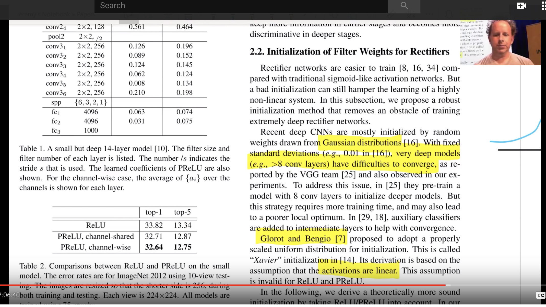
In section 2.2

"Rectifier networks are easier to train"
"Very deep models > 8 conv layers have difficulties to converge"

You may see Glorot initialization (2010). Great paper, and highly influential.

One suggestion to initialize was this one:

So the imagenet folks modified the equation to account for relu

$$\text{std} = \sqrt{\frac{2}{(1 + a^2) \times \text{fan_in}}}$$

# kaiming init / he init for relu
w1 = torch.randn(m,nh)*math.sqrt(2/m)

w1.mean(),w1.std()

(tensor(0.0003), tensor(0.0506))

and now the result is much closer to mean 0, std 1

t = relu(lin(x_valid, w1, b1))
t.mean(),t.std()

(tensor(0.5896), tensor(0.8658))

The paper is worth digging into. Another interesting topic they address is that conv layer is very similar to a matrix multiplication

Then they take you step by step of how the variance changes throughout the network

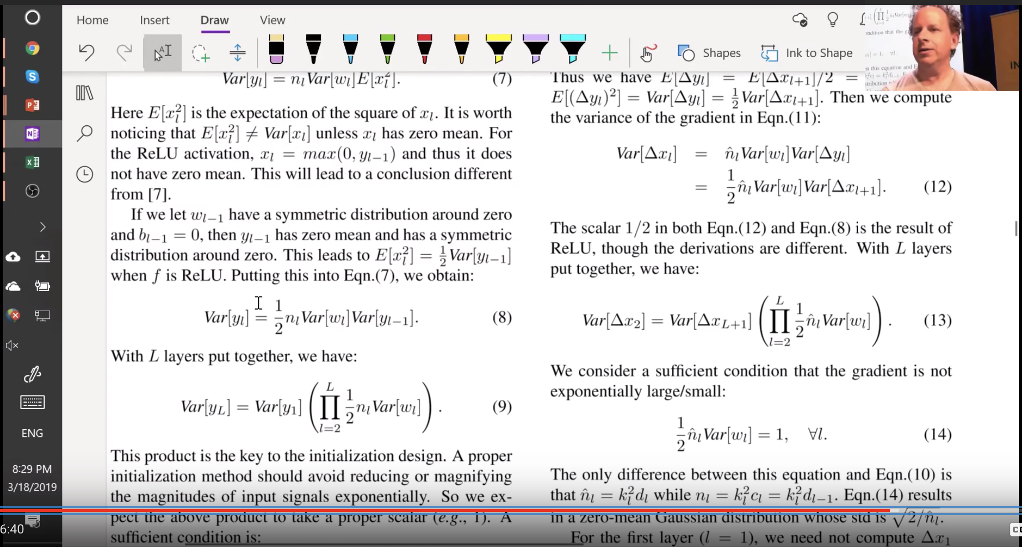
Forward pass is a matrix multiply and backward pass is a matrix multiply with a transpose. And they finally recommend sqrt(2 over activations). Now that we understand how to normalize weights and how to calculate the kaiming normal, lets use the pytorch version of it

#export
from torch.nn import init

w1 = torch.zeros(m,nh)
init.kaiming_normal_(w1, mode='fan_out')
t = relu(lin(x_valid, w1, b1))

Fan in or Fan out

mode: either 'fan_in' (default) or 'fan_out'. Choosing `fan_in`
        preserves the magnitude of the variance of the weights in the
        forward pass. Choosing `fan_out` preserves the magnitudes in the
        backwards pass.

So why are we doing fan_out? Are you dividing by row(m) or by row(nh). BEcause our weight shape is 784 x 50. pytorch actually does the reverse (50 x 784). How does this work?

import torch.nn
torch.nn.Linear(m,nh).weight.shape

    torch.Size([50, 784])

Docstring

torch.nn.Linear.forward??

...
# Source:   
    @weak_script_method
    def forward(self, input):
        return F.linear(input, self.weight, self.bias)
...

In pytorch F always refers to torch.nn.functional

Docstring

torch.nn.functional.linear??

@torch._jit_internal.weak_script
def linear(input, weight, bias=None):
    # type: (Tensor, Tensor, Optional[Tensor]) -> Tensor
    r"""
    Applies a linear transformation to the incoming data: :math:`y = xA^T + b`.

    Shape:

        - Input: :math:`(N, *, in\_features)` where `*` means any number of
          additional dimensions
        - Weight: :math:`(out\_features, in\_features)`
        - Bias: :math:`(out\_features)`
        - Output: :math:`(N, *, out\_features)`
    """
    if input.dim() == 2 and bias is not None:
        # fused op is marginally faster
        ret = torch.addmm(torch.jit._unwrap_optional(bias), input, weight.t())
    else:
        output = input.matmul(weight.t())
        if bias is not None:
            output += torch.jit._unwrap_optional(bias)
        ret = output
    return ret

We see in the doc string that we do the transpose with the following phrase weight.t() and that’s why the dimensions are flipped

What does pytorch do for Conv2d layers?

torch.nn.Conv2d??

Turns out that all the code is passed to another class

#Source:
class Conv2d(_ConvNd):
...

#File:           ~/envs/py3/lib/python3.6/site-packages/torch/nn/modules/conv.py
#Type:           type

So if we dig to the next level of the library

torch.nn.modules.conv._ConvNd.reset_parameters??

# Source:
    def reset_parameters(self):
        n = self.in_channels
        init.kaiming_uniform_(self.weight, a=math.sqrt(5))
        if self.bias is not None:
            fan_in, _ = init._calculate_fan_in_and_fan_out(self.weight)
            bound = 1 / math.sqrt(fan_in)
            init.uniform_(self.bias, -bound, bound)

note that it is divided by math.sqrt(5) which turns out not to perform very well.

Back to activation functions

now we see that the mean is zero and the standard deviation is close to 1

def relu(x): 
    return x.clamp_min(0.) - 0.5


for i in range(10):
    # kaiming init / he init for relu
    w1 = torch.randn(m,nh)*math.sqrt(2./m )
    t1 = relu(lin(x_valid, w1, b1))
    print(t1.mean(), t1.std(), '| ')

tensor(0.0482) tensor(0.7982) | 
tensor(0.0316) tensor(0.8060) | 
tensor(0.1588) tensor(0.9367) | 
tensor(0.0863) tensor(0.8403) | 
tensor(-0.0310) tensor(0.7310) | 
tensor(0.0467) tensor(0.7965) | 
tensor(0.1252) tensor(0.8700) | 
tensor(-0.0610) tensor(0.7189) | 
tensor(0.0264) tensor(0.7755) | 
tensor(0.1081) tensor(0.8605) | 

So where are we now? Fully connected Layers

Our first model

def relu(x): 
    return x.clamp_min(0.) - 0.5

def lin(x, w, b):
    return x@w + b

def model(xb):
    l1 = lin(xb, w1, b1)
    l2 = relu(l1)
    l3 = lin(l2, w2, b2)
    return l3

# timing it on the validation set
%timeit -n 10 _=model(x_valid)

6.71 ms ± 456 µs per loop (mean ± std. dev. of 7 runs, 10 loops each)

assert model(x_valid).shape==torch.Size([x_valid.shape[0],1])

Loss Functions : MSE

We need squeeze() to get rid of that trailing (,1), in order to use mse. (Of course, mse is not a suitable loss function for multi-class classification; we’ll use a better loss function soon. We’ll use mse for now to keep things simple.)

model(x_valid).shape

torch.Size([10000, 1])

#export
def mse(output, targ): 
    # we want to drop the last dimension
    return (output.squeeze(-1) - targ).pow(2).mean()

# converting to float (from tensors)
y_train, y_valid = y_train.float(), y_valid.float()

# make our predictions
preds = model(x_train)
print(preds.shape)

# check our mse
print(mse(preds, y_train))

torch.Size([50000, 1])
tensor(22.1963)

Gradients

How much should you know about matrix calculus? It’s up to you, but there’s a great reference article:

One thing you should learn is the chain rule.

When we are working through our functions, the order works like this:

Then we can simplify to:

y = f(u)

u = g(x)

And then the derivative is:

\frac{dy}{dx} = \frac{dy}{du} \frac{du}{dx}

The representation looks like this:

To do the chain rule, start backwards…

MSE

If we do the derivative of x^2 we get 2x, applying this to the code

#MSE
(output.squeeze(-1) - targ).pow(2).mean()

#MSE grad
inp.g = 2. * (inp.squeeze() - targ).unsqueeze(-1) / inp.shape[0]

Relu

With relu, we know the different gradients, which is either 1 for positive values, or 0 for all others. AS a result, we can easily determine what the relu_grad should be, without a lot of math fuss.

The following math code reads:

(inp>0).float() * out.g

1. if input >0 then True (or 1)
2. if input <=0 then False (or 0)
3. multiply times out.g (which is the gradient

Linear Layer

We do the backwards operation and use the transpose

inp.g = out.g @ w.t()

This is backpropogation

We save intermediate calculations, so we don’t have to calculate twice. As a note, loss is not typically something that is needed in calculating forward and back propogation

def mse_grad(inp, targ): 
    # grad of loss with respect to output of previous layer
    # the derivative of squared output x^2 => 2x
    inp.g = 2. * (inp.squeeze() - targ).unsqueeze(-1) / inp.shape[0]
    
def relu_grad(inp, out):
    # grad of relu with respect to input activations
    inp.g = (inp>0).float() * out.g
    
    
def lin_grad(inp, out, w, b):
    # grad of matmul with respect to input
    inp.g = out.g @ w.t()
    w.g = (inp.unsqueeze(-1) * out.g.unsqueeze(1)).sum(0)
    b.g = out.g.sum(0)
    
def forward_and_backward(inp, targ):
    # forward pass:
    l1 = inp @ w1 + b1
    l2 = relu(l1)
    out = l2 @ w2 + b2
    # we don't actually need the loss in backward!
    loss = mse(out, targ)
    
    # backward pass:
    mse_grad(out, targ)
    lin_grad(l2, out, w2, b2)
    relu_grad(l1, l2)
    lin_grad(inp, l1, w1, b1)

Test and compare vs. pytorch version

forward_and_backward(x_train, y_train)

# Save for testing against later
w1g = w1.g.clone()
w2g = w2.g.clone()
b1g = b1.g.clone()
b2g = b2.g.clone()
ig  = x_train.g.clone()

# =========================================
# PYTORCH version for checking
# =========================================

# check against pytorch's version
xt2 = x_train.clone().requires_grad_(True)
w12 = w1.clone().requires_grad_(True)
w22 = w2.clone().requires_grad_(True)
b12 = b1.clone().requires_grad_(True)
b22 = b2.clone().requires_grad_(True)

def forward(inp, targ):
    # forward pass:
    l1 = inp @ w12 + b12
    l2 = relu(l1)
    out = l2 @ w22 + b22
    # we don't actually need the loss in backward!
    return mse(out, targ)

loss = forward(xt2, y_train)

loss.backward()

test_near(w22.grad, w2g)
test_near(b22.grad, b2g)
test_near(w12.grad, w1g)
test_near(b12.grad, b1g)
test_near(xt2.grad, ig )

Wrapping up

This is a neural network that has all the parts so far, and we’ve written all the pieces

Refactoring

This is very similar to the pytorch API. For each of these functions we combine the forward and backward functions in a single class. Relu will have its own forward and backward functions

__call__ treats the class like a function

class Relu():
    def __call__(self, inp):
        self.inp = inp
        self.out = inp.clamp_min(0.)-0.5
        return self.out
    
    def backward(self):
        self.inp.g = (self.inp>0).float() * self.out.g

As a reminder, in the linear layer Lin we need the gradient of the outputs respect to the weights and outputs respect to the biases

class Lin():
    def __init__(self, w, b): 
        self.w,self.b = w,b
        
    def __call__(self, inp):
        self.inp = inp
        self.out = inp@self.w + self.b
        return self.out
    
    def backward(self):
        self.inp.g = self.out.g @ self.w.t()
        # Creating a giant outer product, just to sum it, is inefficient!
        self.w.g = (self.inp.unsqueeze(-1) * self.out.g.unsqueeze(1)).sum(0)
        self.b.g = self.out.g.sum(0)
        
class Mse():
    def __call__(self, inp, targ):
        self.inp = inp
        self.targ = targ
        self.out = (inp.squeeze() - targ).pow(2).mean()
        return self.out
    
    def backward(self):
        self.inp.g = 2. * (self.inp.squeeze() - self.targ).unsqueeze(-1) / self.targ.shape[0]

Let’s make our model a class as well. There is no pytorch functions or utils used in this class

class Model():
    def __init__(self, w1, b1, w2, b2):
        self.layers = [Lin(w1,b1), Relu(), Lin(w2,b2)]
        self.loss = Mse()
        
    def __call__(self, x, targ):
        for l in self.layers: x = l(x)
        return self.loss(x, targ)
    
    def backward(self):
        self.loss.backward()
        
        # iterates through layers
        for l in reversed(self.layers): 
            l.backward()

Let’s train

# initialize the gradients
w1.g, b1.g, w2.g, b2.g = [None]*4

# create the model
model = Model(w1, b1, w2, b2)

%time loss = model(x_train, y_train)

CPU times: user 274 ms, sys: 44.9 ms, total: 319 ms
Wall time: 59.6 ms

Designing around a generic class with common functions

let’s try and reduce the amount of duplicate code. This will be designed in a generic module class. Then for each function we will extend the base module for each.

• Also will speed up the linear layer using einsum instead of the previous array manipulation

# ============================================
# Base class
# ============================================

class Module():
    def __call__(self, *args):
        self.args = args
        self.out = self.forward(*args)
        return self.out
    
    def forward(self): 
        """ will be implemented when extended"""
        raise Exception('not implemented')
        
    def backward(self): 
        self.bwd(self.out, *self.args)
        
# ============================================
# Relu extended from module class
# ============================================     

class Relu(Module):
    def forward(self, inp): 
        return inp.clamp_min(0.)-0.5
    
    def bwd(self, out, inp): 
        inp.g = (inp>0).float() * out.g
        
# ============================================
# linear layer extended from module class
# ============================================
class Lin(Module):
    def __init__(self, w, b): 
        self.w,self.b = w,b
        
    def forward(self, inp): 
        return inp@self.w + self.b
    
    def bwd(self, out, inp):
        inp.g = out.g @ self.w.t()
        
        # implementing einsum
        self.w.g = torch.einsum("bi,bj->ij", inp, out.g)
        self.b.g = out.g.sum(0)
        
# ============================================
# MSE extended from module
# ============================================
class Mse(Module):
    def forward (self, inp, targ):
        return (inp.squeeze() - targ).pow(2).mean()
    
    def bwd(self, out, inp, targ): 
        inp.g = 2*(inp.squeeze()-targ).unsqueeze(-1) / targ.shape[0]
        
# ============================================
# Remake the model
# ============================================
class Model():
    def __init__(self):
        self.layers = [Lin(w1,b1), Relu(), Lin(w2,b2)]
        self.loss = Mse()
        
    def __call__(self, x, targ):
        for l in self.layers: x = l(x)
        return self.loss(x, targ)
    
    def backward(self):
        self.loss.backward()
        for l in reversed(self.layers): l.backward()

Let’s re-time it again

w1.g,b1.g,w2.g,b2.g = [None]*4
model = Model()

%time loss = model(x_train, y_train)

CPU times: user 294 ms, sys: 11.2 ms, total: 306 ms
Wall time: 44.3 ms

%time model.backward()

CPU times: user 454 ms, sys: 92.4 ms, total: 547 ms
Wall time: 174 ms

Without Einsum

class Lin(Module):
    def __init__(self, w, b): self.w,self.b = w,b
        
    def forward(self, inp): return inp@self.w + self.b
    
    def bwd(self, out, inp):
        inp.g = out.g @ self.w.t()
        self.w.g = inp.t() @ out.g
        self.b.g = out.g.sum(0)

w1.g,b1.g,w2.g,b2.g = [None]*4
model = Model()

%time loss = model(x_train, y_train)

CPU times: user 280 ms, sys: 33.7 ms, total: 314 ms
Wall time: 45.8 ms

%time model.backward()

CPU times: user 442 ms, sys: 70.9 ms, total: 513 ms
Wall time: 158 ms

Pytorch version with nn.Linear and nn.Module

from torch import nn

class Model(nn.Module):
    def __init__(self, n_in, nh, n_out):
        super().__init__()
        self.layers = [nn.Linear(n_in,nh), nn.ReLU(), nn.Linear(nh,n_out)]
        self.loss = mse
        
    def __call__(self, x, targ):
        for l in self.layers: x = l(x)
        return self.loss(x.squeeze(), targ)

model = Model(m, nh, 1)
%time loss = model(x_train, y_train)

CPU times: user 280 ms, sys: 36.7 ms, total: 316 ms
Wall time: 40.5 ms

%time loss.backward()

CPU times: user 183 ms, sys: 6.87 ms, total: 190 ms
Wall time: 33.8 ms