It took me awhile to understand how a pre-trained model could use a different image size than the one it was trained on. I wrote up my notes on using resnet18 for MNIST classification. Maybe they will be helpful to someone.
How does the pre-trained model use our image size? The PyTorch resnet18 model was trained on ImageNet images. These images are 3-channel 224x224 pixels. Our images are 3-channel 28x28. How can we use pre-trained weights for a model trained on different images sizes? Let’s look at the first layers of the model instantiated as learn:
Path: /kaggle/working/data, model=Sequential(
(0): Sequential(
(0): Conv2d(3, 64, kernel_size=(7, 7), stride=(2, 2), padding=(3, 3), bias=False)
(1): BatchNorm2d(64, eps=1e-05, momentum=0.1, affine=True, track_running_stats=True)
(2): ReLU(inplace=True)
(3): MaxPool2d(kernel_size=3, stride=2, padding=1, dilation=1, ceil_mode=False)
(4): Sequential(
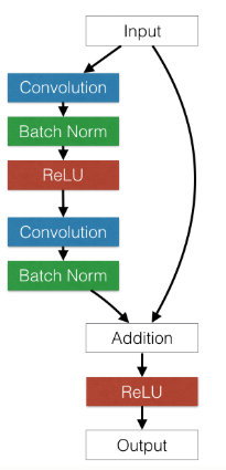
(0): BasicBlock(
(conv1): Conv2d(64, 64, kernel_size=(3, 3), stride=(1, 1), padding=(1, 1), bias=False)
(bn1): BatchNorm2d(64, eps=1e-05, momentum=0.1, affine=True, track_running_stats=True)
(relu): ReLU(inplace=True)
(conv2): Conv2d(64, 64, kernel_size=(3, 3), stride=(1, 1), padding=(1, 1), bias=False)
(bn2): BatchNorm2d(64, eps=1e-05, momentum=0.1, affine=True, track_running_stats=True)
)
:
:
:
The first layer is a 2d convolution. What is a convolution doing? The convolution slides a 7x7 matrix across each input channel of your image and does element-by-element multiplication summed against what it sees (this is sometimes described as matrix multiplication–wrong–or a dot prodcut. The dot product of the stretched out kernel (7x7=49 in this case) and the image segment is the same as element-by-element multuplcation summed). In this model, there are 64 kernels that slide across each channel. A key idea is that the elements of these 7x7 matrices are learned weights. The sizes of the kernels are fixed even though the image sizes are not. This means that the count of weights does not vary at all as a function of image size. This also makes clear why we needed to convert our one channel images to three channels: pre-trained resnet18 requires 3 input channels; these kernels are the weights. In addition to convolutional layers, the model has ReLU layers too. However there are no weights here; this layer is just making some non-linearity of what the prior convolutional layer outputs. So how many weights are there in the first convolutional layer? 7 x 7 x 3 channels x 64 = 9408. At some point though, this logic breaks. At the end of the model, we take the last convolutional layer, connect it to a “fully-connected” layer and output to a certain number of classes. There are two things to understand about this. First let’s look at the actual pre-trained model from the PyTorch website (not our learn instance):
    :
    :
    :
    (1): BasicBlock(
      (conv1): Conv2d(512, 512, kernel_size=(3, 3), stride=(1, 1), padding=(1, 1), bias=False)
      (bn1): BatchNorm2d(512, eps=1e-05, momentum=0.1, affine=True, track_running_stats=True)
      (relu): ReLU(inplace=True)
      (conv2): Conv2d(512, 512, kernel_size=(3, 3), stride=(1, 1), padding=(1, 1), bias=False)
      (bn2): BatchNorm2d(512, eps=1e-05, momentum=0.1, affine=True, track_running_stats=True)
    )
  )
  (avgpool): AdaptiveAvgPool2d(output_size=(1, 1))
  (fc): Linear(in_features=512, out_features=1000, bias=True)
)
The last convolutional block feeds into an AdaptiveAvgPool2d(...) layer which feeds into a fully-connected layer with 1000 outputs. These 1000 outputs are the ImageNet classes. Without going into details, the key idea of the AdaptiveAvgPool2d layer is that it takes any input size and always outputs the same size. This is how we can use any input image size passing through the convolutional layers and make it fit a pre-defined fully-connected layer. However this last layer – this is where our idea breaks down: we don’t have 1000 classes, we have 10. To see how fastai deals with this, let’s look not at the model from the PyTorch website, but the actual model instantiated as learn. When we look at the last layers of this model we see:
    :
    :
    :
     (1): BasicBlock(
        (conv1): Conv2d(512, 512, kernel_size=(3, 3), stride=(1, 1), padding=(1, 1), bias=False)
        (bn1): BatchNorm2d(512, eps=1e-05, momentum=0.1, affine=True, track_running_stats=True)
        (relu): ReLU(inplace=True)
        (conv2): Conv2d(512, 512, kernel_size=(3, 3), stride=(1, 1), padding=(1, 1), bias=False)
        (bn2): BatchNorm2d(512, eps=1e-05, momentum=0.1, affine=True, track_running_stats=True)
      )
    )
  )
  (1): Sequential(
    (0): AdaptiveConcatPool2d(
      (ap): AdaptiveAvgPool2d(output_size=1)
      (mp): AdaptiveMaxPool2d(output_size=1)
    )
    (1): Flatten()
    (2): BatchNorm1d(1024, eps=1e-05, momentum=0.1, affine=True, track_running_stats=True)
    (3): Dropout(p=0.25, inplace=False)
    (4): Linear(in_features=1024, out_features=512, bias=True)
    (5): ReLU(inplace=True)
    (6): BatchNorm1d(512, eps=1e-05, momentum=0.1, affine=True, track_running_stats=True)
    (7): Dropout(p=0.5, inplace=False)
    (8): Linear(in_features=512, out_features=10, bias=True)
  )
Complex! fastai cut off the avgpool and the fc layers from the pre-trained model and then added a bunch of it’s own layers. These added layers are the only ones trained when you first call fit_one_cycle. Notice that out_features=10; fastai made this layer for us based on the number of classes in our data. And that’s it.