DeepLearning-Lec8-Notes

timlee · March 21, 2018, 6:32am

Hi All,

I’m looking forward to the topics in part 2 of deep learning. While I think Jeremy’s notebooks are pretty self-explanatory this week, I’ve uploaded my notes into the forum as well. Hope its helpful!

Tim

Welcome to Lesson 8

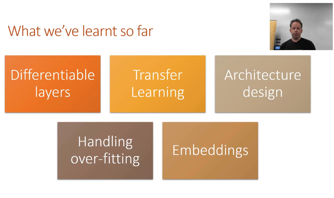
Where we are:

Differentiable Layers - coined by Yann Lecun, we don’t call it deep learning but differentiable programming. In part 1, we setup a diff’able function and a loss function that explains how good the parameters are. If you can define a loss function to score a task, and you have a flexible NN, you are done.

 Yeah, Differentiable Programming is little more than a rebranding of the modern collection Deep Learning techniques, the same way Deep Learning was a rebranding of the modern incarnations of neural nets with more than two layers.
 The important point is that people are now building a new kind of software by assembling networks of parameterized functional blocks and by training them from examples using some form of gradient-based optimization….It’s really very much like a regular program, except it’s parameterized, automatically differentiated, and trainable/optimizable.
 Yann LeCun, Director of FAIR

Transfer Learning - you should never need to start on random data. You should only start if no one has every solved a problem that is remotely close or related to what you are trying to solve. Fastai’s focus is completely focused on transfer learning and as a result the library is much different than any other library. In short, transfer learning takes a trained model, takes away the last few layers, retrains the last few layers, fine tunes the entire architecture, and as a result, trains a lot faster and requires less data!

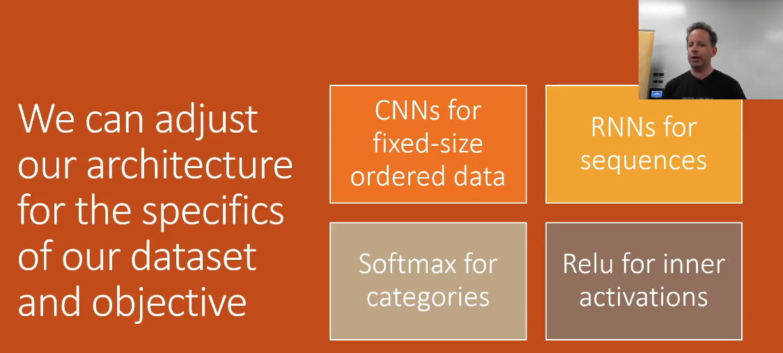
3.Architecture Design - There’s only a few models that generally cover a majority of problems. In part 1, we generally focused on activation functions and the output. We spend less time talking about architecture.

how to Avoid overfitting - Create something that is over-parameterized. Train it for sure, overfit it, which guarantees that there is a predictive capability. Then we use the following techniques to reduce the overfitting to arrive at a generalized model.

Get more data
Data augmentation
Generalized Architecture
regularization
Lastly, reduce architecture complexity

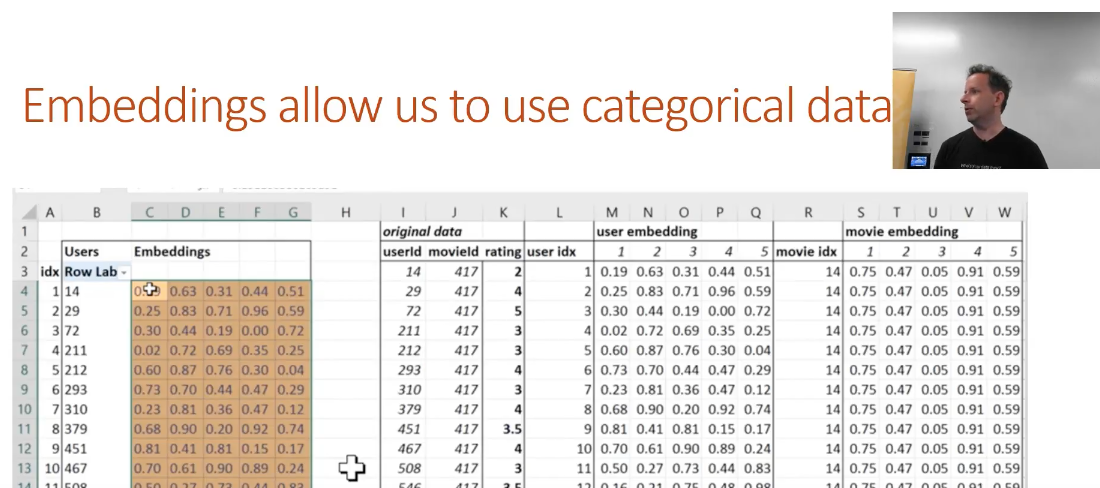
5.Embeddings - Just earlier last year, there was fewer discussions of using embeddings in tabular data (vs. the NLP related topics) Now these days there are more and more examples of using embeddings in traditional structured tabular data settings

Part 2’s Goals / Approach

Part 1 was an introduction to best practices. Overviewed mature techniques that were reasonably reliable for a wide variety of real world problems. These techniques were developed and tested over a longer period of time. Cutting Edge means that the best parameters may not always be evident. It may or may not be the absolute best solution, and the fastai implementation may still be buggy. The techniques covered will be promising in the research world, but may require tweaking. It’s exciting to work with the most current techniques and to also learn these recent techniques and understand what is going on vs. the recipe and pre-built libraries of pytorch and fastai.

Some caveats:

Requires fastai customization
Need to understand python well
Other code resources will generally be research quality
Code samples online nearly have always have problems
Each lesson will be incomplete, ideas to explore

If you are considering building your own box checkout the forums.

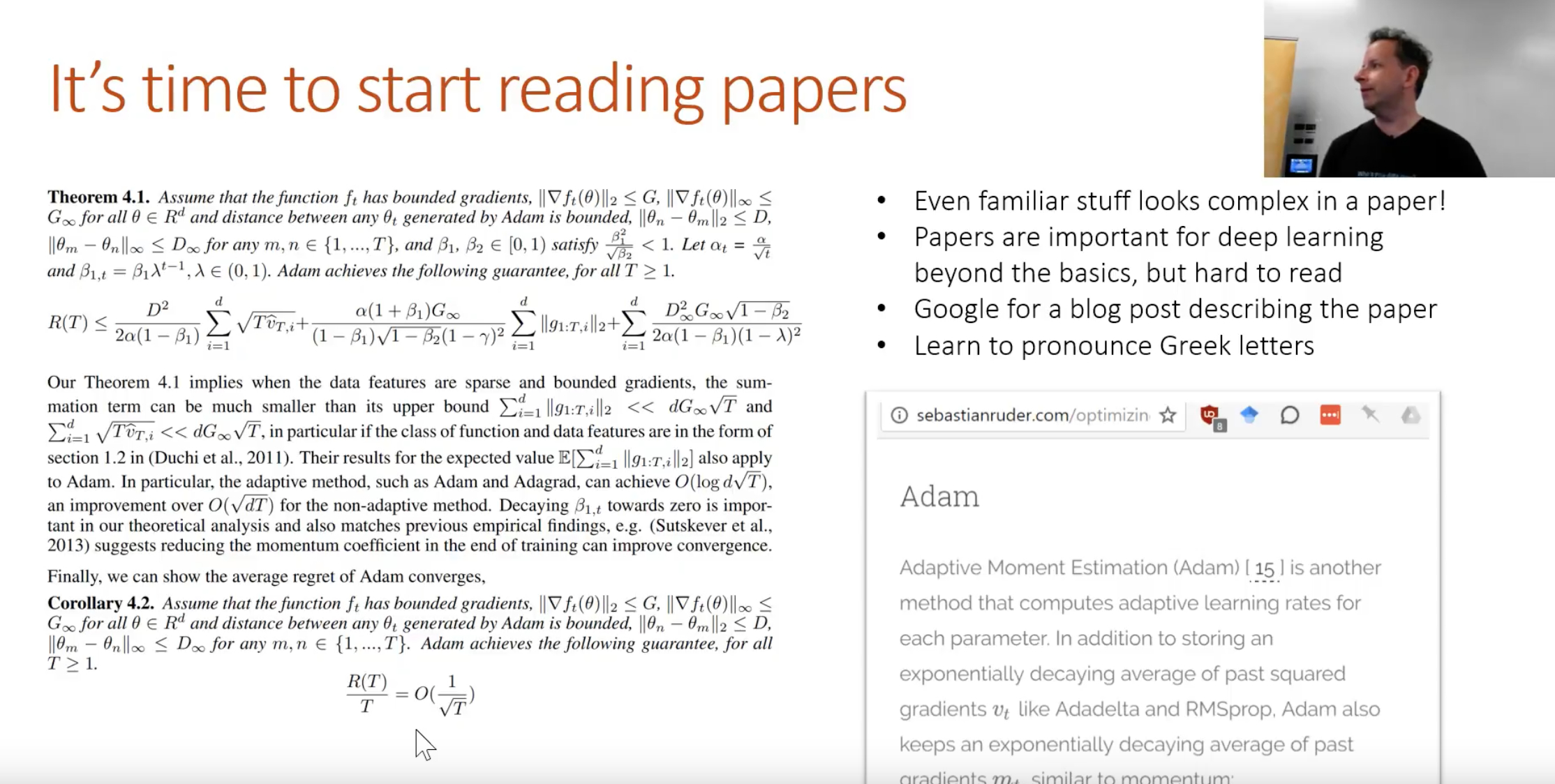
It’s time to start reading papers

Each week we will be implementing a paper. In academic papers love using greek letters. Academics never refactor or substitute, but equations can get very long. Academic papers can be weird, but its the current way that research is commuted these days.

Since this is all cutting-edge, its a great opportunity!

make a blog post, explain things in plain language
maybe a simple implementation that other people can use
use a published case study and translate the technique to a similar problem

Part 2’s Topics

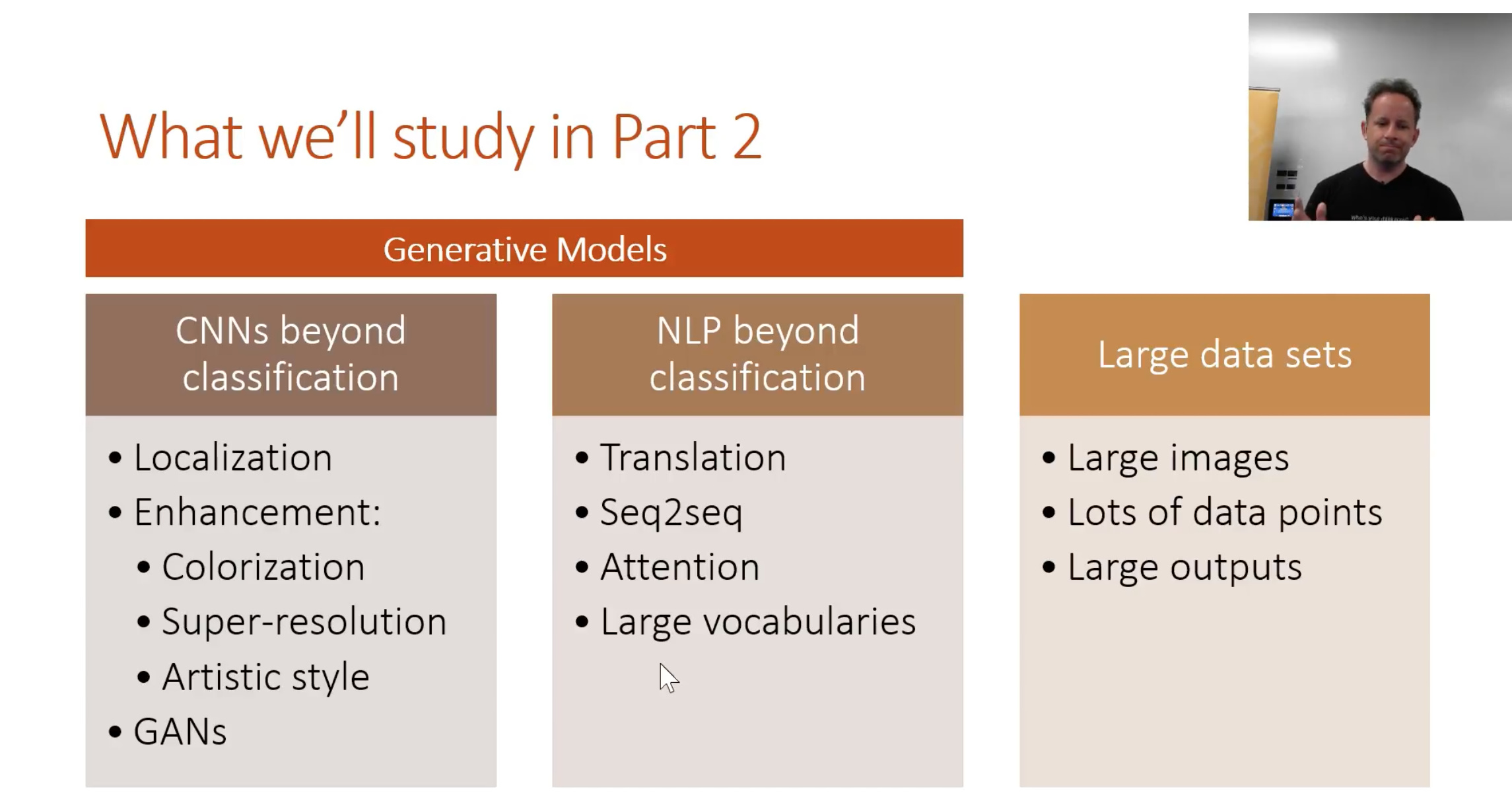
Generative models

NN’s generally output numbers. But now the outputs will be locations of objects, or a complete picture with a class in every pixel. Or an enhanced super-resolution of an image. Or text translated into french. Requires some different ways of thinking about things and different architectures.

Data: Text or Image data

Larger datasets - more objects and size of files

Object Detection

Introduction

1. We are classifying Multiple things

This part is not new, as we have done this in part1, the planet tutorial.

2. Finding Bounding boxes around the objects we are classifying

The box has the object entirely in it, but is no bigger than it needs to be. For these object detection datasets, we are looking for a pool of objects, but not necessarily EVERY object in the photo (mountain, tree cloud).

Stages:

1 Find largest item
2 Find where it is
3 do both at the same time

Stage 1: Find the largest object in the image

Start with the Pascal Notebook

https://github.com/fastai/fastai/blob/master/courses/dl2/pascal.ipynb

%matplotlib inline
%reload_ext autoreload
%autoreload 2

Note, if you have a single GPU change the device to `.set_device(0)`

import sys
sys.path.append('../')
from fastai.conv_learner import *
from fastai.dataset import *

from pathlib import Path
import json
from PIL import ImageDraw, ImageFont
from matplotlib import patches, patheffects

# check to make sure you set the device
torch.cuda.set_device(0)

Pascal VOC

We will be looking at the Pascal VOC dataset. It’s quite slow, so you may prefer to download from this mirror. There are two different competition/research datasets, from 2007 and 2012. We’ll be using the 2007 version. You can use the larger 2012 for better results, or even combine them (but be careful to avoid data leakage between the validation sets if you do this).

Unlike previous lessons, we are using the python 3 standard library pathlib for our paths and file access. pathlib is the python3 library for interacting with files.

The pathlib module was first included in python 3.4 and has been enhanced in each of the subsequent releases. Pathlib is an object oriented interface to the filesystem and provides a more intuitive method to interact with the filesystem in a platform agnostic and pythonic manner.

Cheat Sheet

Note that it returns an OS-specific class (on Linux, PosixPath) so your output may look a little different. Most libraries than take paths as input can take a pathlib object - although some (like cv2) can’t, in which case you can use str() to convert it to a string.

Download the two zips
make a data dir
make a pascal dir
move the .json files out of the PASCAL_VOC into the pascal/ dir

!wget http://pjreddie.com/media/files/VOCtrainval_06-Nov-2007.tar

--2018-03-21 01:00:51--  http://pjreddie.com/media/files/VOCtrainval_06-Nov-2007.tar
Resolving pjreddie.com (pjreddie.com)... 128.208.3.39
Connecting to pjreddie.com (pjreddie.com)|128.208.3.39|:80... connected.
HTTP request sent, awaiting response... 301 Moved Permanently
Location: https://pjreddie.com/media/files/VOCtrainval_06-Nov-2007.tar [following]
--2018-03-21 01:00:51--  https://pjreddie.com/media/files/VOCtrainval_06-Nov-2007.tar
Connecting to pjreddie.com (pjreddie.com)|128.208.3.39|:443... connected.
HTTP request sent, awaiting response... 200 OK
Length: 460032000 (439M) [application/octet-stream]
Saving to: ‘VOCtrainval_06-Nov-2007.tar’

VOCtrainval_06-Nov- 100%[===================>] 438.72M  12.7MB/s    in 28s     

2018-03-21 01:01:20 (15.5 MB/s) - ‘VOCtrainval_06-Nov-2007.tar’ saved [460032000/460032000]

!wget https://storage.googleapis.com/coco-dataset/external/PASCAL_VOC.zip

--2018-03-21 01:05:31--  https://storage.googleapis.com/coco-dataset/external/PASCAL_VOC.zip
Resolving storage.googleapis.com (storage.googleapis.com)... 172.217.6.48, 2607:f8b0:4005:805::2010
Connecting to storage.googleapis.com (storage.googleapis.com)|172.217.6.48|:443... connected.
HTTP request sent, awaiting response... 200 OK
Length: 1998182 (1.9M) [application/zip]
Saving to: ‘PASCAL_VOC.zip’

PASCAL_VOC.zip      100%[===================>]   1.91M  --.-KB/s    in 0.02s   

2018-03-21 01:05:31 (77.5 MB/s) - ‘PASCAL_VOC.zip’ saved [1998182/1998182]

We will be using Python3’s path lib, creating a generator around the directory

PATH = Path('data/pascal')
list(PATH.iterdir())

[PosixPath('data/pascal/VOCdevkit'),
 PosixPath('data/pascal/pascal_train2007.json'),
 PosixPath('data/pascal/pascal_test2007.json'),
 PosixPath('data/pascal/pascal_val2012.json'),
 PosixPath('data/pascal/VOCtrainval_06-Nov-2007.tar'),
 PosixPath('data/pascal/pascal_val2007.json'),
 PosixPath('data/pascal/PASCAL_VOC.zip'),
 PosixPath('data/pascal/pascal_train2012.json'),
 PosixPath('data/pascal/PASCAL_VOC'),
 PosixPath('data/pascal/models'),
 PosixPath('data/pascal/src'),
 PosixPath('data/pascal/tmp')]

Load the annotations

trn_j = json.load((PATH/'pascal_train2007.json').open())
trn_j.keys()

dict_keys(['images', 'type', 'annotations', 'categories'])

Image information

filename - the related image with filename
height - how big the height of the image is
width - how big the width of the image is
id - the image id for joining to other datasets

IMAGES,ANNOTATIONS,CATEGORIES = ['images', 'annotations', 'categories']
trn_j[IMAGES][:5]

[{'file_name': '000012.jpg', 'height': 333, 'id': 12, 'width': 500},
 {'file_name': '000017.jpg', 'height': 364, 'id': 17, 'width': 480},
 {'file_name': '000023.jpg', 'height': 500, 'id': 23, 'width': 334},
 {'file_name': '000026.jpg', 'height': 333, 'id': 26, 'width': 500},
 {'file_name': '000032.jpg', 'height': 281, 'id': 32, 'width': 500}]

Bounding Boxes

bbox: column, row (top left) , height, width
id: which image
category_id : which label
segmentation : ignore of this tutorail (polygon bounding

trn_j[ANNOTATIONS][:2]

[{'area': 34104,
  'bbox': [155, 96, 196, 174],
  'category_id': 7,
  'id': 1,
  'ignore': 0,
  'image_id': 12,
  'iscrowd': 0,
  'segmentation': [[155, 96, 155, 270, 351, 270, 351, 96]]},
 {'area': 13110,
  'bbox': [184, 61, 95, 138],
  'category_id': 15,
  'id': 2,
  'ignore': 0,
  'image_id': 17,
  'iscrowd': 0,
  'segmentation': [[184, 61, 184, 199, 279, 199, 279, 61]]}]

Make a lookup from id to name

trn_j[CATEGORIES][:4]

[{'id': 1, 'name': 'aeroplane', 'supercategory': 'none'},
 {'id': 2, 'name': 'bicycle', 'supercategory': 'none'},
 {'id': 3, 'name': 'bird', 'supercategory': 'none'},
 {'id': 4, 'name': 'boat', 'supercategory': 'none'}]

It’s helpful to use constants instead of strings, since we get tab-completion and don’t mistype.

FILE_NAME,ID,IMG_ID,CAT_ID,BBOX = 'file_name','id','image_id','category_id','bbox'

cats = dict((o[ID], o['name']) for o in trn_j[CATEGORIES])
trn_fns = dict((o[ID], o[FILE_NAME]) for o in trn_j[IMAGES])
trn_ids = [o[ID] for o in trn_j[IMAGES]]

Lets take a look at whats in the VOC 2007 dataset

list((PATH/'VOCdevkit'/'VOC2007').iterdir())

[PosixPath('data/pascal/VOCdevkit/VOC2007/ImageSets'),
 PosixPath('data/pascal/VOCdevkit/VOC2007/SegmentationObject'),
 PosixPath('data/pascal/VOCdevkit/VOC2007/SegmentationClass'),
 PosixPath('data/pascal/VOCdevkit/VOC2007/Annotations'),
 PosixPath('data/pascal/VOCdevkit/VOC2007/JPEGImages')]

Store the Image path

JPEGS = 'VOCdevkit/VOC2007/JPEGImages'

Make a compound path

IMG_PATH = PATH/JPEGS
list(IMG_PATH.iterdir())[:5]

[PosixPath('data/pascal/VOCdevkit/VOC2007/JPEGImages/006948.jpg'),
 PosixPath('data/pascal/VOCdevkit/VOC2007/JPEGImages/005796.jpg'),
 PosixPath('data/pascal/VOCdevkit/VOC2007/JPEGImages/007006.jpg'),
 PosixPath('data/pascal/VOCdevkit/VOC2007/JPEGImages/004693.jpg'),
 PosixPath('data/pascal/VOCdevkit/VOC2007/JPEGImages/002279.jpg')]

Each image has a unique ID.

im0_d = trn_j[IMAGES][0]
im0_d[FILE_NAME],im0_d[ID]

('000012.jpg', 12)

A defaultdict is useful any time you want to have a default dictionary entry for new keys. Here we create a dict from image IDs to a list of annotations (tuple of bounding box and class id).

We convert VOC’s height/width into top-left/bottom-right, and switch x/y coords to be consistent with numpy.
We are swapping dimensions, to be consistent, numpy, ROWS x COLUMNS

Output

{
    IMG_ID  : (array(top_left_row, top_left_col, lower_right_row, lower_right_col), CAT_ID)
}

#initialize the default dictionary
trn_anno = collections.defaultdict(lambda:[])

# for each annotation
for o in trn_j[ANNOTATIONS]:
    
    # if not ignore
    if not o['ignore']:
        # get the original bounding box information
        bb = o[BBOX]
        bb = np.array([bb[1], bb[0], bb[3]+bb[1]-1, bb[2]+bb[0]-1])
        
        # 
        trn_anno[o[IMG_ID]].append((bb,o[CAT_ID]))
        
len(trn_anno)

example 1

im0_a = im_a[0]; im0_a

(array([ 96, 155, 269, 350]), 7)

cats[7]

'car'

example 2

trn_anno[17]

[(array([ 61, 184, 198, 278]), 15), (array([ 77,  89, 335, 402]), 13)]

cats[15],cats[13]

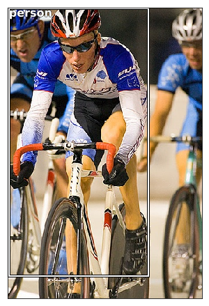
('person', 'horse')

Create a short function that will change a boundbox to height & width to translate data

def bb_hw(a): return np.array([a[1],a[0],a[3]-a[1],a[2]-a[0]])

We will use fast.ai’s open_image library to create an image to view

im = open_image(IMG_PATH/im0_d[FILE_NAME])

Create a short function to show the image in the notebook

Matplotlib’s plt.subplots is a really useful wrapper for creating plots, regardless of whether you have more than one subplot. Note that Matplotlib has an optional object-oriented API which I think is much easier to understand and use (although few examples online use it!)

def show_img(im, figsize=None, ax=None):
    if not ax: fig,ax = plt.subplots(figsize=figsize)
    ax.imshow(im)
    ax.get_xaxis().set_visible(False)
    ax.get_yaxis().set_visible(False)
    return ax

Create an outlining function

A simple but rarely used trick to making text visible regardless of background is to use white text with black outline, or visa versa. Here’s how to do it in matplotlib.

def draw_outline(o, lw):
    o.set_path_effects([patheffects.Stroke(
        linewidth=lw, foreground='black'), patheffects.Normal()])

Note that * in argument lists is the splat operator. In this case it’s a little shortcut compared to writing out b[-2],b[-1].

Make a rectangle for the bounding box

def draw_rect(ax, b):
    patch = ax.add_patch(patches.Rectangle(b[:2], *b[-2:], fill=False, edgecolor='white', lw=2))
    draw_outline(patch, 4)

Make a quick function to write the text label (for the category)

def draw_text(ax, xy, txt, sz=14):
    text = ax.text(*xy, txt,
        verticalalignment='top', color='white', fontsize=sz, weight='bold')
    draw_outline(text, 1)

Let’s test out showing an image!

ax = show_img(im)
b = bb_hw(im0_a[0])
draw_rect(ax, b)
draw_text(ax, b[:2], cats[im0_a[1]])

output_51_0

Let’s make a function to show multiple objects on a single image

def draw_im(im, ann):
    ax = show_img(im, figsize=(16,8))
    for b,c in ann:
        b = bb_hw(b)
        draw_rect(ax, b)
        draw_text(ax, b[:2], cats[c], sz=16)

def draw_idx(i):
    im_a = trn_anno[i]
    im = open_image(IMG_PATH/trn_fns[i])
    print(im.shape)
    draw_im(im, im_a)

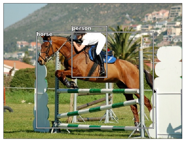
draw_idx(17)

(364, 480, 3)

output_55_1

Next Complex step - Largest Item Classifier

A lambda function is simply a way to define an anonymous function inline. Here we use it to describe how to sort the annotation for each image - by bounding box size (descending).

This snippet sorts the objets

sorted(b, key=lambda x: np.product(x[0][-2:]-x[0][:2]), reverse=True)

We subtract the upper left from the bottom right and multiply (np.product) the values to get an area.
lambda x: np.product(x[0][-2:]-x[0][:2])

def get_lrg(b):
    if not b: raise Exception()
    b = sorted(b, key=lambda x: np.product(x[0][-2:]-x[0][:2]), reverse=True)
    return b[0]

dictionary comprehension - storing the biggest objects:

{
    IMG_ID : largest bounding box,
    ...
}

trn_lrg_anno = {a: get_lrg(b) for a,b in trn_anno.items()}

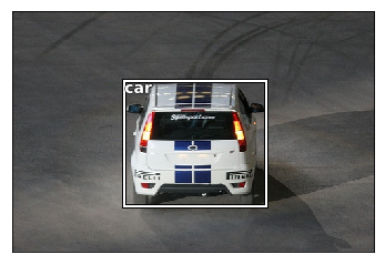
b,c = trn_lrg_anno[23]
b = bb_hw(b)
ax = show_img(open_image(IMG_PATH/trn_fns[23]), figsize=(5,10))
draw_rect(ax, b)
draw_text(ax, b[:2], cats[c], sz=16)

output_60_0

Let’s store the largest object per file in a `CSV` file

(PATH/'tmp').mkdir(exist_ok=True)
CSV = PATH/'tmp/lrg.csv'

Often it’s easiest to simply create a CSV of the data you want to model, rather than trying to create a custom dataset. Here we use Pandas to help us create a CSV of the image filename and class.

df = pd.DataFrame({'fn': [trn_fns[o] for o in trn_ids],
                   'cat': [cats[trn_lrg_anno[o][1]] for o in trn_ids]}, columns=['fn','cat'])
df.to_csv(CSV, index=False)

Make a Resnet model to learn

Considerations

The training images are different sized
Since we are doing bounding boxes, many of the objects are near the edge, so we want to be careful not to cut the objects off the picture
So we will put CropType.NO so we will “squish” instead

f_model = resnet34
sz=224
bs=64

From here it’s just like Dogs vs Cats!

tfms = tfms_from_model(f_model, sz, aug_tfms=transforms_side_on, crop_type=CropType.NO)
md = ImageClassifierData.from_csv(PATH, JPEGS, CSV, tfms=tfms)

A note on Data Loaders

A data loader is an iterator that will provide a mini-batch of data ( subset). But first we need to ensure that we start at the beginning of the dataset. Pythons’ iter() method will create an iterator object and start at the beginning of the dataset. And afterwards our iterator will have __next__ that can be used to pull a mini-batch

md.trn_dl

<fastai.dataloader.DataLoader at 0x7fba10572908>

Let’s look at a single example

x,y=next(iter(md.val_dl))

Some observations

not a numpy array
not on the CPU
[torch.cuda.FloatTensor of size 2x3x224x224 (GPU 0)] shape is wrong
not numbers between 0 and 1

x[:2]

( 0 , 0 ,.,.) = 
  3.9125e-01  4.3014e-01  4.8172e-01  ...   1.7518e-01  3.2367e-01  4.0783e-01
  5.1636e-01  4.4973e-01  5.9202e-01  ...   1.7386e-01  2.3164e-01  3.6722e-01
  5.4416e-01  5.7267e-01  7.0099e-01  ...   5.7682e-02  2.2320e-01  3.5455e-01
                 ...                   ⋱                   ...                
  1.4604e+00  1.5029e+00  1.5195e+00  ...   7.8030e-01  5.6716e-01 -6.3922e-01
  9.3739e-01  1.0210e+00  1.1599e+00  ...   1.1281e+00  1.0895e+00  4.5857e-01
  5.8584e-01  4.5245e-01  2.9605e-01  ...   1.0003e+00  9.2495e-01  8.2729e-01

( 0 , 1 ,.,.) = 
  2.4041e-01  3.1444e-01  4.1422e-01  ...   3.3162e-01  4.7052e-01  5.4764e-01
  3.9737e-01  4.2156e-01  5.7304e-01  ...   3.3887e-01  3.8799e-01  5.2038e-01
  5.2462e-01  5.8245e-01  6.7485e-01  ...   2.5190e-01  4.0003e-01  5.1502e-01
                 ...                   ⋱                   ...                
  1.4721e+00  1.5019e+00  1.5077e+00  ...   6.0917e-01  4.4337e-01 -7.3978e-01
  8.4169e-01  9.4566e-01  1.0678e+00  ...   9.7373e-01  1.0164e+00  3.9674e-01
  4.7731e-01  3.6442e-01  1.8230e-01  ...   8.5592e-01  8.5008e-01  7.5529e-01

( 0 , 2 ,.,.) = 
  6.3094e-01  7.6758e-01  9.1924e-01  ...   4.6997e-01  5.8218e-01  6.3571e-01
  8.6685e-01  8.9343e-01  1.0892e+00  ...   4.5970e-01  4.9210e-01  6.0825e-01
  9.6684e-01  1.0009e+00  1.0785e+00  ...   3.5109e-01  5.0631e-01  6.3579e-01
                 ...                   ⋱                   ...                
  1.5606e+00  1.5927e+00  1.6055e+00  ...   5.4531e-01  3.8118e-01 -7.9327e-01
  9.2625e-01  1.0206e+00  1.1445e+00  ...   9.1826e-01  9.3747e-01  3.1286e-01
  5.6966e-01  4.4559e-01  2.6428e-01  ...   8.0080e-01  7.7093e-01  6.7405e-01
      ⋮  

( 1 , 0 ,.,.) = 
  2.1343e+00  2.1323e+00  2.1205e+00  ...  -2.0870e+00 -2.0843e+00 -2.0837e+00
  2.1703e+00  2.1498e+00  2.1186e+00  ...  -2.0939e+00 -2.0863e+00 -2.0861e+00
  2.1454e+00  2.1375e+00  2.0940e+00  ...  -2.0922e+00 -2.0923e+00 -2.0933e+00
                 ...                   ⋱                   ...                
 -1.8905e+00 -1.8818e+00 -1.8374e+00  ...  -1.8581e+00 -1.8778e+00 -1.8109e+00
 -1.8530e+00 -1.8759e+00 -1.8143e+00  ...  -1.8267e+00 -1.8599e+00 -1.8636e+00
 -1.8764e+00 -1.8944e+00 -1.9561e+00  ...  -1.8202e+00 -1.7856e+00 -1.8230e+00

( 1 , 1 ,.,.) = 
  2.2305e+00  2.1392e+00  1.7919e+00  ...  -2.0042e+00 -2.0013e+00 -2.0007e+00
  2.2569e+00  2.1649e+00  1.8062e+00  ...  -2.0112e+00 -2.0034e+00 -2.0032e+00
  2.2407e+00  2.1826e+00  1.8103e+00  ...  -2.0095e+00 -2.0096e+00 -2.0105e+00
                 ...                   ⋱                   ...                
 -1.8032e+00 -1.7944e+00 -1.7489e+00  ...  -1.7557e+00 -1.7819e+00 -1.7218e+00
 -1.7649e+00 -1.7883e+00 -1.7254e+00  ...  -1.7107e+00 -1.7613e+00 -1.7757e+00
 -1.7888e+00 -1.8072e+00 -1.8703e+00  ...  -1.7174e+00 -1.6914e+00 -1.7343e+00

( 1 , 2 ,.,.) = 
  1.8575e+00  1.3323e+00  6.5693e-01  ...  -1.7730e+00 -1.7702e+00 -1.7696e+00
  1.9155e+00  1.3577e+00  6.7138e-01  ...  -1.7800e+00 -1.7723e+00 -1.7721e+00
  1.8913e+00  1.3744e+00  6.8420e-01  ...  -1.7783e+00 -1.7784e+00 -1.7794e+00
                 ...                   ⋱                   ...                
 -1.5730e+00 -1.5642e+00 -1.5189e+00  ...  -1.5329e+00 -1.5559e+00 -1.4919e+00
 -1.5348e+00 -1.5581e+00 -1.4955e+00  ...  -1.4945e+00 -1.5366e+00 -1.5456e+00
 -1.5586e+00 -1.5769e+00 -1.6397e+00  ...  -1.4945e+00 -1.4639e+00 -1.5043e+00
[torch.cuda.FloatTensor of size 2x3x224x224 (GPU 0)]

imagenet_stats = A([0.485, 0.456, 0.406], [0.229, 0.224, 0.225])
inception_stats = A([0.5, 0.5, 0.5], [0.5, 0.5, 0.5])
inception_models = (inception_4, inceptionresnet_2)    

def tfms_from_stats(stats, sz, aug_tfms=None, max_zoom=None, pad=0, crop_type=CropType.RANDOM,
                    tfm_y=None, sz_y=None, pad_mode=cv2.BORDER_REFLECT):
    if aug_tfms is None: aug_tfms=[]
    ----------------------------------------------- NOTE THE MANIPULATION ----------------------------------
    tfm_norm = Normalize(*stats, tfm_y=tfm_y)
    tfm_denorm = Denormalize(*stats)
    ----------------------------------------------- NOTE THE MANIPULATION ----------------------------------
    val_crop = CropType.CENTER if crop_type==CropType.RANDOM else crop_type
    val_tfm = image_gen(tfm_norm, tfm_denorm, sz, pad=pad, crop_type=val_crop, tfm_y=tfm_y, sz_y=sz_y)
    trn_tfm=image_gen(tfm_norm, tfm_denorm, sz, tfms=aug_tfms, max_zoom=max_zoom,
                      pad=pad, crop_type=crop_type, tfm_y=tfm_y, sz_y=sz_y, pad_mode=pad_mode)
    return trn_tfm, val_tfm

show_img(md.val_ds.denorm(to_np(x))[0]);

output_76_0

Using Resnet 34

Get a pretrained learner

learn = ConvLearner.pretrained(f_model, md, metrics=[accuracy])
learn.opt_fn = optim.Adam

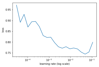
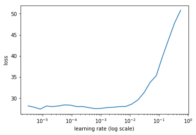
Find a learning rate

lrf=learn.lr_find(1e-5,100)

Failed to display Jupyter Widget of type HBox.

If you're reading this message in the Jupyter Notebook or JupyterLab Notebook, it may mean that the widgets JavaScript is still loading. If this message persists, it likely means that the widgets JavaScript library is either not installed or not enabled. See the Jupyter Widgets Documentation for setup instructions.

If you're reading this message in another frontend (for example, a static rendering on GitHub or NBViewer), it may mean that your frontend doesn't currently support widgets.

 78%|███████▊  | 25/32 [00:08<00:02,  2.84it/s, loss=14.9]

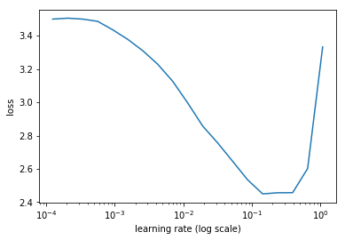
learn.sched.plot()

output_81_0

to change the truncation of the plot use the command below

learn.sched.plot(n_skip=5, n_skip_end=1)

output_83_0

Set the learning rate

lr = 2e-2

learn.fit(lr, 1, cycle_len=1)

Failed to display Jupyter Widget of type HBox.

If you're reading this message in the Jupyter Notebook or JupyterLab Notebook, it may mean that the widgets JavaScript is still loading. If this message persists, it likely means that the widgets JavaScript library is either not installed or not enabled. See the Jupyter Widgets Documentation for setup instructions.

If you're reading this message in another frontend (for example, a static rendering on GitHub or NBViewer), it may mean that your frontend doesn't currently support widgets.

epoch      trn_loss   val_loss   accuracy                 
    0      1.280753   0.604127   0.806941  






[0.60412693, 0.8069411069154739]

lrs = np.array([lr/1000,lr/100,lr])

We freeze all layers except the last two layers, find new learning rate and retrain

learn.freeze_to(-2)

lrf=learn.lr_find(lrs/1000)
learn.sched.plot(1)

Failed to display Jupyter Widget of type HBox.

If you're reading this message in the Jupyter Notebook or JupyterLab Notebook, it may mean that the widgets JavaScript is still loading. If this message persists, it likely means that the widgets JavaScript library is either not installed or not enabled. See the Jupyter Widgets Documentation for setup instructions.

If you're reading this message in another frontend (for example, a static rendering on GitHub or NBViewer), it may mean that your frontend doesn't currently support widgets.

 84%|████████▍ | 27/32 [00:08<00:01,  3.26it/s, loss=3.45]

output_90_2

learn.fit(lrs/5, 1, cycle_len=1)

Failed to display Jupyter Widget of type HBox.

If you're reading this message in the Jupyter Notebook or JupyterLab Notebook, it may mean that the widgets JavaScript is still loading. If this message persists, it likely means that the widgets JavaScript library is either not installed or not enabled. See the Jupyter Widgets Documentation for setup instructions.

If you're reading this message in another frontend (for example, a static rendering on GitHub or NBViewer), it may mean that your frontend doesn't currently support widgets.

epoch      trn_loss   val_loss   accuracy                  
    0      0.777971   0.556964   0.832782  






[0.5569643, 0.8327824547886848]

Accuracy is still at 83%

learn.unfreeze()

Accuracy isn’t improving much - since many images have multiple different objects, it’s going to be impossible to be that accurate.

learn.fit(lrs/5, 1, cycle_len=2)

Failed to display Jupyter Widget of type HBox.

If you're reading this message in the Jupyter Notebook or JupyterLab Notebook, it may mean that the widgets JavaScript is still loading. If this message persists, it likely means that the widgets JavaScript library is either not installed or not enabled. See the Jupyter Widgets Documentation for setup instructions.

If you're reading this message in another frontend (for example, a static rendering on GitHub or NBViewer), it may mean that your frontend doesn't currently support widgets.

epoch      trn_loss   val_loss   accuracy                  
    0      0.676254   0.546998   0.834285  
    1      0.460609   0.533741   0.833233                  






[0.53374064, 0.8332331702113152]

learn.save('clas_one')

learn.load('clas_one')

x,y = next(iter(md.val_dl))
probs = F.softmax(predict_batch(learn.model, x), -1)
x,preds = to_np(x),to_np(probs)
preds = np.argmax(preds, -1)

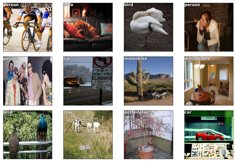
Let’s look at the 20 classes

fig, axes = plt.subplots(3, 4, figsize=(12, 8))
for i,ax in enumerate(axes.flat):
    ima=md.val_ds.denorm(x)[i]
    b = md.classes[preds[i]]
    ax = show_img(ima, ax=ax)
    draw_text(ax, (0,0), b)
plt.tight_layout()

Clipping input data to the valid range for imshow with RGB data ([0..1] for floats or [0..255] for integers).

Note on debuggers

You can use the python debugger pdb to step through code.

pdb.set_trace() to set a breakpoint
%debug magic to trace an error

Commands you need to know:

s / n / c
u / d
p
l

> <ipython-input-99-6d7dd6a3d3cc>(4)<module>()
-> ima=md.val_ds.denorm(x)[i]
(Pdb) h

Documented commands (type help <topic>):
========================================
EOF    c          d        h         list      q        rv       undisplay
a      cl         debug    help      ll        quit     s        unt      
alias  clear      disable  ignore    longlist  r        source   until    
args   commands   display  interact  n         restart  step     up       
b      condition  down     j         next      return   tbreak   w        
break  cont       enable   jump      p         retval   u        whatis   
bt     continue   exit     l         pp        run      unalias  where    

Miscellaneous help topics:
==========================
exec  pdb

Can view variables throughout the debugging process

(Pdb) n # will go to next step

(Pdb) l # will show the currentlocation
  1  	fig, axes = plt.subplots(3, 4, figsize=(12, 8))
  2  	for i,ax in enumerate(axes.flat):
  3  	    pdb.set_trace()
  4  ->	    ima=md.val_ds.denorm(x)[i]
  5  	    b = md.classes[preds[i]]
  6  	    ax = show_img(ima, ax=ax)
  7  	    draw_text(ax, (0,0), b)
  8  	plt.tight_layout()
[EOF]

(Pdb) s # will go into a function

(Pdb) c # continue to next break point

Next Stage : Create a bounding box around an object

We know we can make a regression nn instead of a classification. This is accomplished by changing the last layer of the NN. Instead of Softmax, and use MSE, it is now a regression problem. We can have multiple outputs.

So what we will do is a multiple regression to predict the following values:

top left x
top left y
lower right x
lower right y

But what about the loss function?

BB_CSV = PATH/'tmp/bb.csv'

Transform the bounding box data

bb = np.array([trn_lrg_anno[o][0] for o in trn_ids])
bbs = [' '.join(str(p) for p in o) for o in bb]

df = pd.DataFrame({'fn': [trn_fns[o] for o in trn_ids], 'bbox': bbs}, columns=['fn','bbox'])
df.to_csv(BB_CSV, index=False)

BB_CSV.open().readlines()[:5]

['fn,bbox\n',
 '000012.jpg,96 155 269 350\n',
 '000017.jpg,77 89 335 402\n',
 '000023.jpg,1 2 461 242\n',
 '000026.jpg,124 89 211 336\n']

Set our model and parameters

f_model=resnet34
sz=224
bs=64

Tell `fast.ai` to make a continous network model

Set continuous=True to tell fastai this is a regression problem, which means it won’t one-hot encode the labels, and will use MSE as the default crit.

Note that we have to tell the transforms constructor that our labels are coordinates, so that it can handle the transforms correctly.

Also, we use CropType.NO because we want to ‘squish’ the rectangular images into squares, rather than center cropping, so that we don’t accidentally crop out some of the objects. (This is less of an issue in something like imagenet, where there is a single object to classify, and it’s generally large and centrally located).

tfms = tfms_from_model(f_model, sz, crop_type=CropType.NO, tfm_y=TfmType.COORD)
md = ImageClassifierData.from_csv(PATH, JPEGS, BB_CSV, tfms=tfms, continuous=True)

x,y=next(iter(md.val_dl))

ima=md.val_ds.denorm(to_np(x))[0]
b = bb_hw(to_np(y[0])); b

array([ 49.,   0., 131., 205.], dtype=float32)

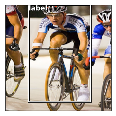
Let’s look at an example image with box

ax = show_img(ima)
draw_rect(ax, b)
draw_text(ax, b[:2], 'label')

output_115_0

How add additional layers on the end of the Resnet (`custom head`)

fastai let’s you use a custom_head to add your own module on top of a convnet, instead of the adaptive pooling and fully connected net which is added by default. In this case, we don’t want to do any pooling, since we need to know the activations of each grid cell.

The final layer has 4 activations, one per bounding box coordinate. Our target is continuous, not categorical, so the MSE loss function used does not do any sigmoid or softmax to the module outputs.

head_reg4 = nn.Sequential(Flatten(), nn.Linear(25088,4))
learn = ConvLearner.pretrained(f_model, md, custom_head=head_reg4)
learn.opt_fn = optim.Adam
learn.crit = nn.L1Loss()

Check the Model to see that the additional layer has been addedm

# learn.summary()

OrderedDict([('Conv2d-1',
              OrderedDict([('input_shape', [-1, 3, 224, 224]),
                           ('output_shape', [-1, 64, 112, 112]),
                           ('trainable', False),
                           ('nb_params', 9408)])),
              ....
              ....
             ('ReLU-121',
              OrderedDict([('input_shape', [-1, 512, 7, 7]),
                           ('output_shape', [-1, 512, 7, 7]),
                           ('nb_params', 0)])),
             ('BasicBlock-122',
              OrderedDict([('input_shape', [-1, 512, 7, 7]),
                           ('output_shape', [-1, 512, 7, 7]),
                           ('nb_params', 0)])),
             ('Flatten-123',
              OrderedDict([('input_shape', [-1, 512, 7, 7]),
                           ('output_shape', [-1, 25088]),
                           ('nb_params', 0)])),
                           
             ------------------- New layer ------------------------
             ('Linear-124',
              OrderedDict([('input_shape', [-1, 25088]),
                           ('output_shape', [-1, 4]),
                           ('trainable', True),
                           ('nb_params', 100356)]))])
             ------------------- New layer ------------------------

Try and fit the model

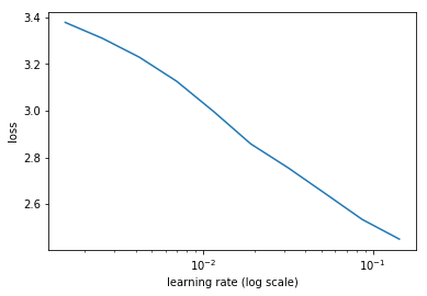
learn.lr_find(1e-5,100)
learn.sched.plot(5)

Failed to display Jupyter Widget of type HBox.

If you're reading this message in the Jupyter Notebook or JupyterLab Notebook, it may mean that the widgets JavaScript is still loading. If this message persists, it likely means that the widgets JavaScript library is either not installed or not enabled. See the Jupyter Widgets Documentation for setup instructions.

If you're reading this message in another frontend (for example, a static rendering on GitHub or NBViewer), it may mean that your frontend doesn't currently support widgets.

 78%|███████▊  | 25/32 [00:04<00:01,  5.36it/s, loss=475]

output_123_2

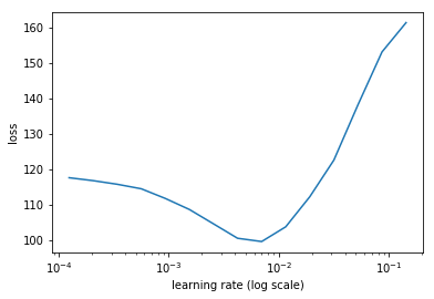
Set the learning rate

lr = 2e-3

Train

learn.fit(lr, 2, cycle_len=1, cycle_mult=2)

Failed to display Jupyter Widget of type HBox.

If you're reading this message in the Jupyter Notebook or JupyterLab Notebook, it may mean that the widgets JavaScript is still loading. If this message persists, it likely means that the widgets JavaScript library is either not installed or not enabled. See the Jupyter Widgets Documentation for setup instructions.

If you're reading this message in another frontend (for example, a static rendering on GitHub or NBViewer), it may mean that your frontend doesn't currently support widgets.

epoch      trn_loss   val_loss                            
    0      50.135777  34.477402 
    1      37.689602  29.124092                           
    2      31.387475  27.658106                           






[27.658106]

lrs = np.array([lr/100,lr/10,lr])

learn.freeze_to(-2)

lrf=learn.lr_find(lrs/1000)
learn.sched.plot(1)

Failed to display Jupyter Widget of type HBox.

If you're reading this message in the Jupyter Notebook or JupyterLab Notebook, it may mean that the widgets JavaScript is still loading. If this message persists, it likely means that the widgets JavaScript library is either not installed or not enabled. See the Jupyter Widgets Documentation for setup instructions.

If you're reading this message in another frontend (for example, a static rendering on GitHub or NBViewer), it may mean that your frontend doesn't currently support widgets.

epoch      trn_loss   val_loss                            
    0      80.37384   175370041032704.0

output_130_2

learn.fit(lrs, 2, cycle_len=1, cycle_mult=2)

Failed to display Jupyter Widget of type HBox.

If you're reading this message in the Jupyter Notebook or JupyterLab Notebook, it may mean that the widgets JavaScript is still loading. If this message persists, it likely means that the widgets JavaScript library is either not installed or not enabled. See the Jupyter Widgets Documentation for setup instructions.

If you're reading this message in another frontend (for example, a static rendering on GitHub or NBViewer), it may mean that your frontend doesn't currently support widgets.

epoch      trn_loss   val_loss                            
    0      25.814654  23.127014 
    1      21.655237  21.125538                           
    2      17.600573  20.209145                           






[20.209145]

learn.freeze_to(-3)

learn.fit(lrs, 1, cycle_len=2)

Failed to display Jupyter Widget of type HBox.

If you're reading this message in the Jupyter Notebook or JupyterLab Notebook, it may mean that the widgets JavaScript is still loading. If this message persists, it likely means that the widgets JavaScript library is either not installed or not enabled. See the Jupyter Widgets Documentation for setup instructions.

If you're reading this message in another frontend (for example, a static rendering on GitHub or NBViewer), it may mean that your frontend doesn't currently support widgets.

epoch      trn_loss   val_loss                            
    0      16.644847  21.78323  
    1      14.667386  20.380457                           






[20.380457]

Save our Model

learn.save('reg4')

learn.load('reg4')

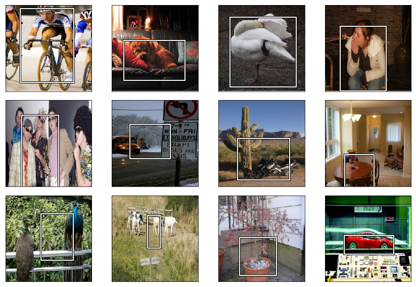
Let’s see how our model did!

Anytime there’s a single subject, our model does decent. When there’s multiple objects our model doesn’t perform as well. Next week we will improve our model

x,y = next(iter(md.val_dl))
learn.model.eval()
preds = to_np(learn.model(VV(x)))

fig, axes = plt.subplots(3, 4, figsize=(12, 8))
for i,ax in enumerate(axes.flat):
    ima=md.val_ds.denorm(to_np(x))[i]
    b = bb_hw(preds[i])
    ax = show_img(ima, ax=ax)
    draw_rect(ax, b)
plt.tight_layout()

Clipping input data to the valid range for imshow with RGB data ([0..1] for floats or [0..255] for integers).

yggg · March 21, 2018, 8:02am

Wow, Thank you for summerizing that! May I suggest to add references to video timestamps, if only that’s not too much work? Regardlessly, this work is superb!

TonyHoldroyd · March 21, 2018, 12:02pm

Thanks for doing that, it must have taken a while, very useful.

init_27 · March 21, 2018, 1:14pm

Our saviour @timlee is back.

jeremy · March 21, 2018, 1:35pm

There’s already time-stamped links in the main in-class discussion post.

jeremy · March 21, 2018, 1:37pm

Many thanks for the great notes @timlee. One correction: open_image is from fastai, not PIL. Underneath it uses opencv (cv2) . It’s the function we looked at the implementation of in vscode.

A clarification: pathlib isn’t just for creating a generator - that’s what the iterdir method does. pathlib does a lot more (e.g the / operator, the open method we used to open the json file, etc).

amritv · March 21, 2018, 2:20pm

@timlee really glad to see your notes again. Thanks!

A_TF57 · March 21, 2018, 5:59pm

This is great! As always, thanks for putting these together @timlee

mandroid6 · March 21, 2018, 7:00pm

After working through the week’s notebook ones after going through my notes, and then a second pass along with your notes always helps in bolstering the conceptual understanding.

@timlee really a big thanks to you from us all for compiling and explaining the lessons again in such detail!

avinash3593 · March 22, 2018, 2:51am

Thanks for the notes @timlee. As usual, it’s detailed and useful.

timlee · March 22, 2018, 5:37am

Thanks for the feedback. I’ve updated the text according!

Interogativ · March 22, 2018, 11:10pm

It’s all greek to me.

Posted this here because I’m not sure where the wiki is for this lesson. But anyway ,here’s a pretty good link for both Greek and Mathematical notation.
https://www.rapidtables.com/math/symbols/Basic_Math_Symbols.html

jeremy · March 22, 2018, 11:27pm

You can edit the ‘in class discussion’ post.

Interogativ · March 23, 2018, 12:50am

did that, should I withdraw the post?

jeremy · March 23, 2018, 4:01am

No need - it’s nice to have both I think.

evgeny · March 23, 2018, 4:23pm

Thank you for putting it together @timlee! That’s very helpful.

kro · March 23, 2018, 8:00pm

Does anyone know where predict_batch is defined?

It’s used in these notes where the model is tested under “Largest item classifier” in

probs = F.softmax(predict_batch(learn.model, x), -1)

I tried jupyter notebook’s shift-tab and ?predict_batch, as well as googling and also just trying grep -R for it in the fastai dir in bash, but no luck.

adrian · March 24, 2018, 11:26am

Its a function in fastai.model. Try out using VS Code as Jeremy was showing in the lecture, very useful for digging around in the source code.

suvash · March 24, 2018, 1:10pm

You probably haven’t updated(git pull) fastai repo.
Also, easily searchable on Github. https://github.com/fastai/fastai/search?utf8=✓&q=predict_batch&type=

SHAR1 · March 24, 2018, 7:10pm

You can try this out !

DeepLearning-Lec8-Notes

Welcome to Lesson 8

Where we are:

Part 2’s Goals / Approach

Some caveats:

It’s time to start reading papers

Since this is all cutting-edge, its a great opportunity!

Part 2’s Topics

Generative models

Data: Text or Image data

Larger datasets - more objects and size of files

Object Detection

Introduction

1. We are classifying Multiple things

2. Finding Bounding boxes around the objects we are classifying

Stages:

Stage 1: Find the largest object in the image

Start with the Pascal Notebook

Note, if you have a single GPU change the device to .set_device(0)

Pascal VOC

We will be using Python3’s path lib, creating a generator around the directory

Load the annotations

Image information

Bounding Boxes

Make a lookup from id to name

Lets take a look at whats in the VOC 2007 dataset

Store the Image path

Make a compound path

example 1

example 2

Create a short function that will change a boundbox to height & width to translate data

Create a short function to show the image in the notebook

Create an outlining function

Make a rectangle for the bounding box

Make a quick function to write the text label (for the category)

Let’s test out showing an image!

Let’s make a function to show multiple objects on a single image

Next Complex step - Largest Item Classifier

dictionary comprehension - storing the biggest objects:

Let’s store the largest object per file in a CSV file

Make a Resnet model to learn

Considerations

A note on Data Loaders

Let’s look at a single example

Some observations

Using Resnet 34

Find a learning rate

to change the truncation of the plot use the command below

Set the learning rate

We freeze all layers except the last two layers, find new learning rate and retrain

Accuracy is still at 83%

Let’s look at the 20 classes

Note on debuggers

Next Stage : Create a bounding box around an object

But what about the loss function?

Transform the bounding box data

Set our model and parameters

Tell fast.ai to make a continous network model

Let’s look at an example image with box

How add additional layers on the end of the Resnet (custom head)

Check the Model to see that the additional layer has been addedm

Try and fit the model

Set the learning rate

Train

Save our Model

Let’s see how our model did!

Note, if you have a single GPU change the device to `.set_device(0)`

Let’s store the largest object per file in a `CSV` file

Tell `fast.ai` to make a continous network model

How add additional layers on the end of the Resnet (`custom head`)