My best attempt at capturing all the detail from tonight’s talk. Ran into trouble trying to actually run the GPU code. If someone got the rest of the lesson to work, I can try and compile notes together for something more comprehensive. For now, here’s what I got. Hope it is helpful.
Unofficial Deep Learning Lecture 1 Notes
Started talking about logistics
Talking about the forums (which crashed right when he ran it)
What is Machine Learning?
Anything instead of programming a computer step by step, you provide examples instead. Arthur Samuels. Talking about breast cancer survivors. Can work really well, depends on the experts and if you can come up with the features.
In the last few years…
It’s become more advanced, can recommend pre-written responses. Can actually generate responses.
- Google suggest responses.
- human can sketch, and the deep learning can turn that into a painting of any style. Newer versions can update the painting real-time.
- How is Deep learning being used at Google?
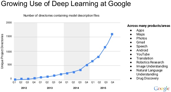
Deep Learning improves cooling techniques
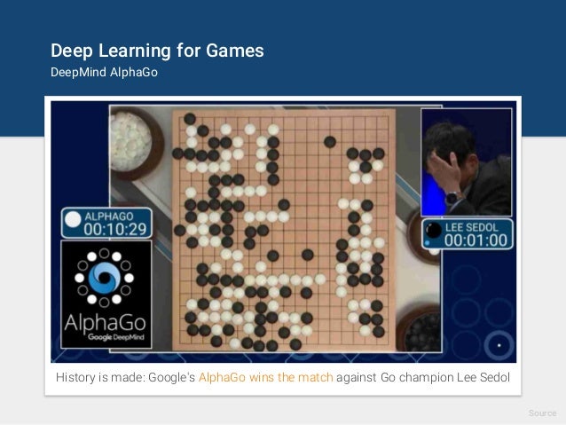
Deep Learning AlphaGo
We are looking for a flexible math function that we can solve any problem. If its infinitely flexible, then there will be many many parameters. So to ensure that it works, we need to ensure that fitting those variables needs to be fast and scalable.
Earlier AlphaGO used images of the go-board itself in winning and non-winning situation and applied CNN onto them. (Now, state of the art reinforcement learning is used).
Key Element: Neural Network
The functional form is the neural network.
Key Element 2: Gradient Descent
There are much recent optimization algorithms than gradient descent but we continue to use GD because in high dimensional space, gradient descent gives almost the same minima (as other algorithm’s), so it doesn’t really matter which algorithm we use for learning parameters.
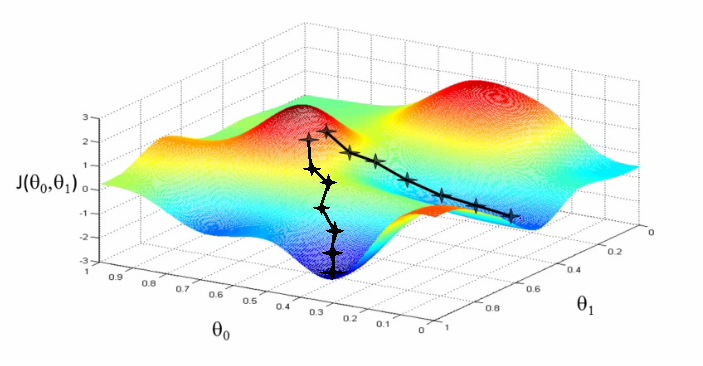
This is how we optimize and move towards the optimal solution for all variables simultaneously. Below as a visual approach for a 2D search. J is considered the loss. We want the local minima. The two thetas are two input parameters.
Very simple models of Gradient Descent + Neural Networks usually work out the best
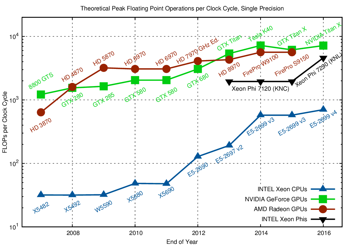
Key Element 3: Next Advance: GPUs
Convolutional Neural Networks
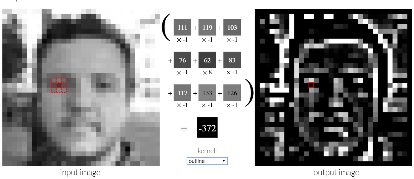
http://setosa.io/ev/image-kernels/
Play with the interactive website (you can even upload your own photo or video) and customize your own kernel by changing the matrix values to manipulate one image to another.
**discussion ** - multiply pixel by numbers to get another set of pixels. The below example 3 x 3 is a ‘top edge detector’
import numpy as np

A = np.matrix ('1 2 1; 0 0 0; -1 -2 -1')
A
matrix([[ 1,  2,  1],
        [ 0,  0,  0],
        [-1, -2, -1]])
What about a right edge detector?
import numpy as np

A = np.matrix ('-1 0 1; -2 0 2; -1 0 1')
A
matrix([[-1, 0, 1],
        [-2, 0, 2],
        [-1, 0, 1]])
We are not doing a matrix product, we are doing element wise multiplication followed by addition.
What if you stacked all of these together in a linear combination?
Not very interesting.
**What if we used non-linear functions (sigmoid) ? ** turns out if we do a single layer, and we feed these linear operations through a non-linearity, and repeat that over and over again to represent a wide variety of problems.
Then we will “learn” the matrices necessary.
Most common non linear unit : ReLU or Rectified Linear Unit
- Max of (0, value)
- Cutting edge element
Gradient Descent
Sample of the different Layers of the Convolutional Neural Network
Layer 1 - edges
Layer 2 - color + shapes
Layer 5 - large complexity
http://blog.xiax.ai/2017/09/01/DNN-overview-and-Linear-model-with-CNN-features/layers%20of%20DNN.png
Big Idea: Cycle Multiply + Add, replace negatives with zeros, Multiply + add replac…
Example Time ( Hour 2 Mark) - transition to Crestle
https://s.users.crestle.com/.../notebooks/courses/fastai/deeplearning1/nbs/lesson1.ipynb
Using Convolutional Neural Networks
Welcome to the first week of the first deep learning certificate! We’re going to use convolutional neural networks (CNNs) to allow our computer to see - something that is only possible thanks to deep learning.
Introduction to this week’s task: ‘Dogs vs Cats’
We’re going to try to create a model to enter the Dogs vs Cats competition at Kaggle. There are 25,000 labelled dog and cat photos available for training, and 12,500 in the test set that we have to try to label for this competition. According to the Kaggle web-site, when this competition was launched (end of 2013): “State of the art: The current literature suggests machine classifiers can score above 80% accuracy on this task”. So if we can beat 80%, then we will be at the cutting edge as of 2013!
First, replace the default Keras with version 1.2.2. This is needed for part 1 of the course.
# Put these at the top of every notebook, to get automatic reloading and inline plotting
%reload_ext autoreload
%autoreload 2
%matplotlib inline
# This file contains all the main external libs we'll use

import sys
sys.path.append('/Users/tlee010/Desktop/github_repos/fastai/')
from fastai.imports import *
from fastai.transforms import *
from fastai.conv_learner import *
from fastai.model import *
from fastai.dataset import *
from fastai.sgdr import *
from fastai.plots import *
PATH = "/Users/tlee010/Desktop/MSAN-pywork/DeepLearning/"
How to look at functions
?
For example, use ? in front of the ImageClassifierData function to review the function’s parameters. Alternatively, highlight the function, and press Shift+Tab.
??
For example, use ?? in front of the ImageClassifierData function to review the source code.
Getting the Data of cats and dogs
!wget http://files.fast.ai/data/dogscats.zip
--2017-10-30 20:36:22--  http://files.fast.ai/data/dogscats.zip
Resolving files.fast.ai... 67.205.15.147
Connecting to files.fast.ai|67.205.15.147|:80... connected.
HTTP request sent, awaiting response... 200 OK
Length: 857214334 (818M) [application/zip]
Saving to: ‘dogscats.zip’

dogscats.zip        100%[===================>] 817.50M  6.93MB/s    in 2m 29s

2017-10-30 20:38:51 (5.50 MB/s) - ‘dogscats.zip’ saved [857214334/857214334]
Unzip in same folder
!unzip dogscats.zip
First look at cat pictures
Our library will assume that you have train and valid directories. It also assumes that each directory will have subdirectories for each class you wish to recognize (in this case, ‘cats’ and ‘dogs’).
PATH = "/Users/tlee010/Desktop/MSAN-pywork/DeepLearning/dogscats/"
!ls {PATH}
e[1me[36mmodelse[me[m e[1me[36msamplee[me[m e[1me[36mtest1e[me[m e[1me[36mtraine[me[m e[1me[36mvalide[me[m
files = !ls {PATH}valid/cats | head
files
['cat.1001.jpg',
 'cat.10016.jpg',
 'cat.10026.jpg',
 'cat.10048.jpg',
 'cat.10050.jpg',
 'cat.10064.jpg',
 'cat.10071.jpg',
 'cat.10091.jpg',
 'cat.10103.jpg',
 'cat.10104.jpg']
img = plt.imread(f'{PATH}valid/cats/{files[0]}')
plt.imshow(img);
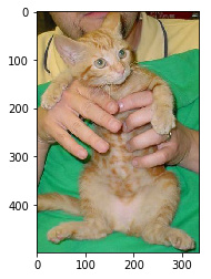
img.shape
(499, 336, 3)
img[:4,:4]
array([[[60, 58, 10],
        [60, 57, 14],
        [61, 56, 18],
        [63, 54, 23]],

       [[56, 54,  6],
        [56, 53, 10],
        [57, 52, 14],
        [60, 51, 20]],

       [[52, 49,  4],
        [52, 49,  6],
        [53, 48, 10],
        [56, 47, 16]],

       [[50, 47,  2],
        [50, 47,  4],
        [51, 45,  9],
        [53, 44, 13]]], dtype=uint8)
Use ResNet 34, its generally the better library
The learning rate determines how quickly or how slowly you want to update the weights (or parameters). Learning rate is one of the most difficult parameters to set, because it significantly affect model performance.
The method learn.lr_find() helps you find an optimal learning rate. It uses the technique developed in the 2015 paper Cyclical Learning Rates for Training Neural Networks, where we simply keep increasing the learning rate from a very small value, until the loss starts decreasing. We can plot the learning rate across batches to see what this looks like.
We first create a new learner, since we want to know how to set the learning rate for a new (untrained) model.
Let’s run the Model!
sz=224
%%time
data = ImageClassifierData.from_paths(PATH, tfms=tfms_from_model(resnet34, sz))
learn = ConvLearner.pretrained(resnet34, data, precompute=True)
learn.fit(0.01, 1)
Downloading: “https://download.pytorch.org/models/resnet34-333f7ec4.pth” to /home/nbuser/.torch/models/resnet34-333f7ec4.pth
100%|██████████| 87306240/87306240 [00:02<00:00, 33445235.94it/s]
100%|██████████| 360/360 [01:58<00:00, 3.03it/s]
100%|██████████| 32/32 [00:10<00:00, 3.07it/s]
Choosing a learning rate
Number of Epochs
How many times should it go through the pictures to learn the different features.
Learning Rate
With gradient descent - you have to figure out which way is downhill. We take the derivative up hill or downhill. The learning rate is what do we multiple the derivative (gradient by). You might overshoot if you go too large, but if you go small, you might take forever to get there.
lrf=learn.lr_find()
Better to find a learning rate
There’s a function for it in fastai library
??learn.lr_find()
['/bin/bash: -c: line 1: syntax error: unexpected end of file']
learn.lr_find()
How it works
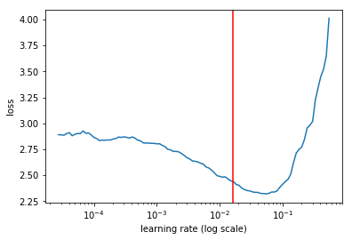
It uses mini-batches to calculate the learning rate, and then we can make a plot between error vs. learning rate. You want to choose a learning rate where the error doesn’t increase anymore.
learn.sched.plot_lr()
When choosing a learning rate with the LR finder, you can plot a vertical line to ensure you choose the correct x-coordinate of the point you’re interested in. Otherwise it can be difficult to interpret values on the x-axis, since they’re in log scale.
import matplotlib.pyplot as plt
learn.sched.plot()
plt.axvline(x=1.6e-2, color="red");

