Here are some CNN activations for Starry Night. If you’ve visualized activations, please post some here so others can see.
You can click an image to zoom in. You can click the zoomed-in image to zoom in once more.
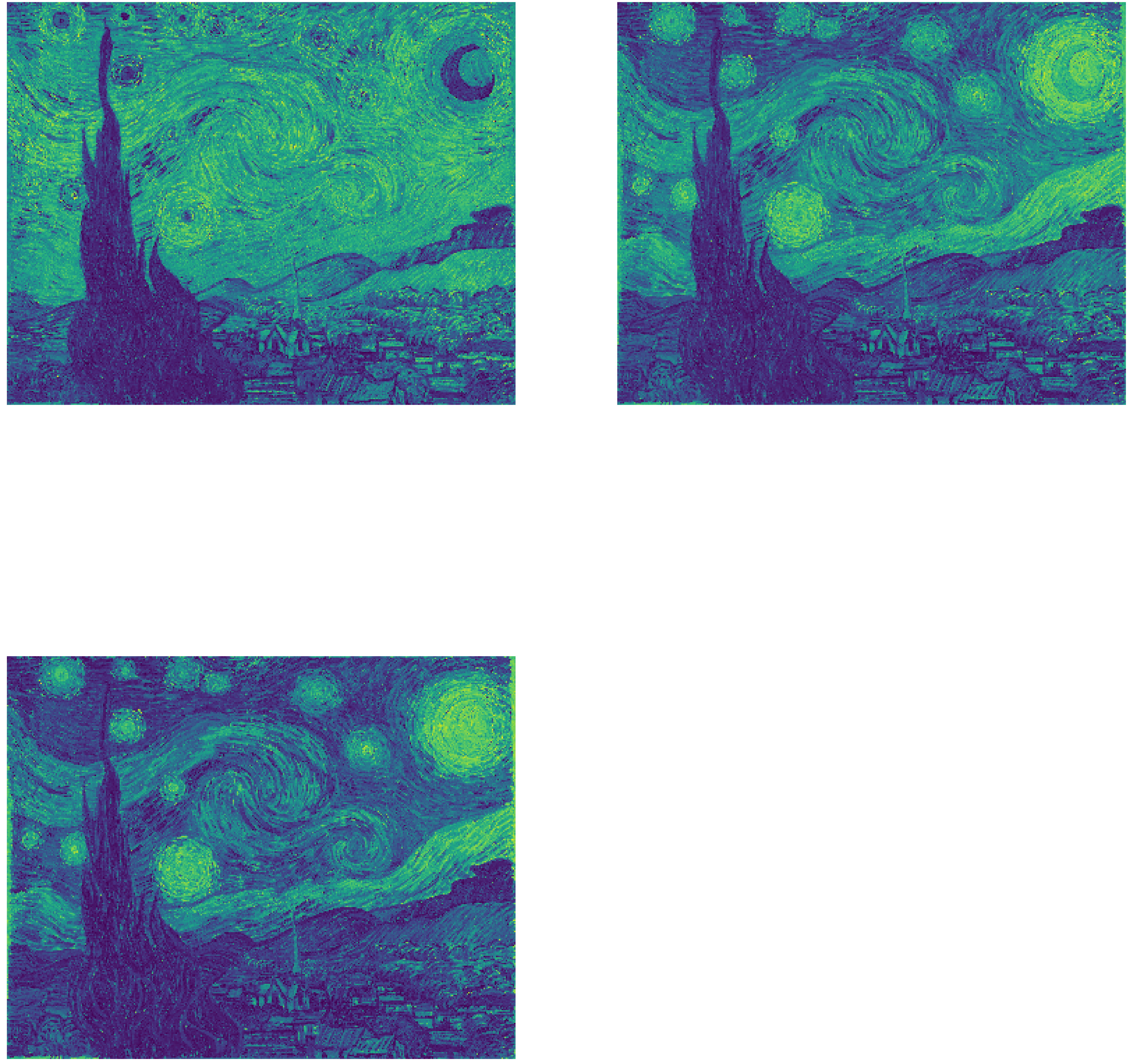
Input (three color channels)
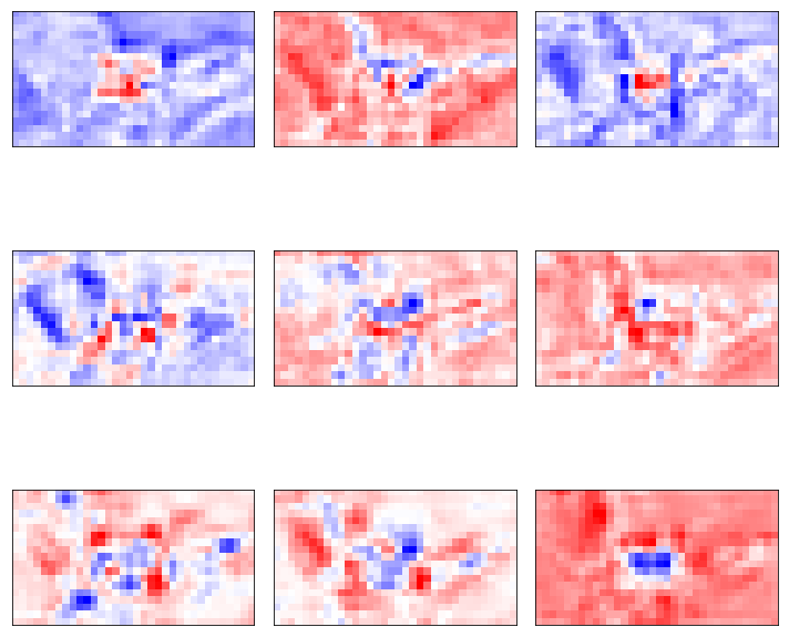
block1_conv1 (64 filters) (first conv layer)

Each filter is latching on to different parts of the image.
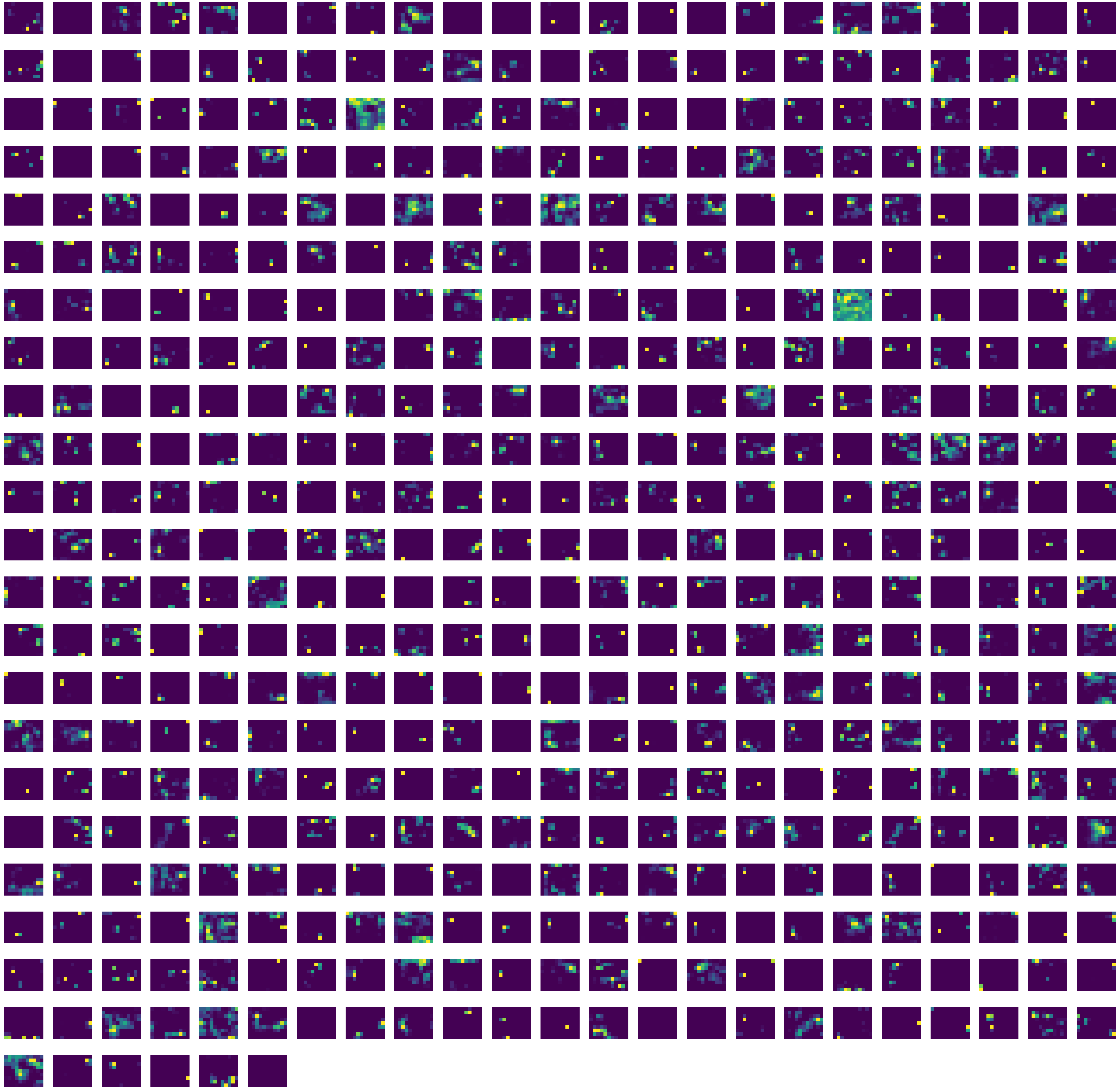
block5_pool (512 filters) (last layer)
A portion of block5_pool (40 out of 512 filters) (top left)
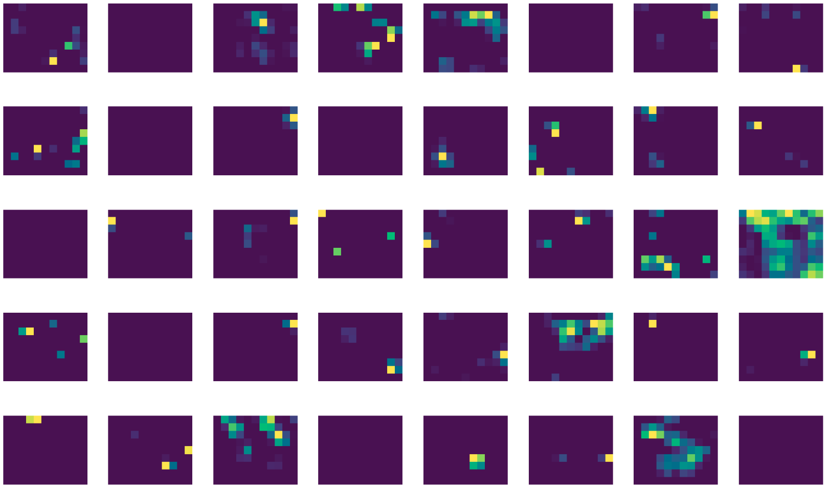
These filter activations are very simple, yet each colored block corresponds to the activations of previous layers which had complicated-looking activations. I want to say, “each colored block is rich with information”, but I don’t know if that makes sense. I do wonder what each colored block means, though.
#Here’s a link to all the filter results on one page
Code
def plots(ims, figsize=(12,6), rows=1, cols=None, interp=None, titles=None, cmap=None):
    f = plt.figure(figsize=figsize)
    for i in range(len(ims)):
        sp = f.add_subplot(rows, cols, i+1)
        if titles is not None:
            sp.set_title(titles[i], fontsize=18)
        plt.imshow(ims[i], interpolation=interp, cmap=cmap)
        plt.axis('off') # New
        plt.subplots_adjust(hspace = 0.500) # New
    return f

# preprocess the image
style_image = Image.open('data/starry_night.jpg')
style_image = style_image.resize(np.divide(style_image.size, 3.5).astype('int32'))
style_arr = preproc(np.expand_dims(style_image ,0)[:,:,:,:3])
shp = style_arr.shape

# Get the activations
start = time()
model = VGG16_Avg(include_top=False, input_shape=shp[1:])
to_plot = []
for layer in model.layers:
    layer = layer.output
    layer_model = Model(model.input, layer)
    # get activations
    activations = layer_model.predict(style_arr)
    images = []
    h, w, f = activations[0].shape
    for k in range(f): # for each filter
        image = []
        for i in range(h): # for each row
            for j in range(w): # for each column
                pixel = activations[0][i][j][k]
                image.append(pixel)
        images.append(np.array(image).reshape(h, w))
    to_plot.append(images)
print(time() - start) # 24 seconds elapsed

# Plot the activations and save the plots
squares = np.array([i**2 for i in range(24)])
start = time()
for i, layer in enumerate(model.layers):
    start2 = time()
    try:
        images = to_plot[i]
        nb_imgs = len(images)
        nb_rows = np.sqrt([square for square in squares if square >= nb_imgs][0]).astype('int')
        fig = plots(images, rows=nb_rows, cols=nb_rows, figsize=(96,96))
        plt.savefig("data/starry_night/%s.png" % layer.name, bbox_inches='tight')
    except ValueError:
        print(i, nb_imgs, nb_rows)
        break
    print(layer.name+':', time() - start2)
print(time() - start) # 9 minutes, 21 seconds elapsed