*Most words are in English.
Important
This guide assumes a basic understanding of derivatives and matrices.

You can view a more neatly formatted version of this post on my blog.
Backpropagation sounds and looks daunting. It doesn’t need to be. In fact, backpropagation is really just a fancy word for the chain rule. Implementing a backpropagation algorithm is simply implementing one big fat chain rule equation.
Let’s remind ourselves of the chain rule. The chain rule lets us figure out how much a given variable indirectly changes with respect to another variable. Take the example below.
We want to figure out how much y changes with each increment in x. The problem is that x doesn’t direcly change y. Rather, x changes u which in turn changes y.
The chain rule allows us to solve this problem. In this case, the chain rule tells us that we can figure out how much x indirecly changes y by multiplying the derivative of y with respect to u, and the derivative of u with respect to x.
Aaand I’ve just described backpropagation in a nutshell. That’s all there really is to it. The only difference is that in a neural network there are many more intermediate variables and functions, and that we want to find out how the weights indirectly change the loss.
Let’s see this tangibly in action.
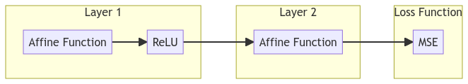
We have the following neural network comprised of two layers: the first layer contains the affine function[1] together with the ReLU, while the second layer contains only the affine function. The loss, which is MSE (Mean Squared Error), will then be calculated from the output of the second layer.
Mathematically speaking, the first layer with a single sample x looks like this.
The second layer looks like this.
And the loss function looks like this.
Note
MSE in its most basic form looks like this.
\text{MSE} = \frac{(y - x)^2}{1}If we have multiple data points, then it looks like this.
\text{MSE} = \frac{(y_1 - x_1)^2+(y_2 - x_2)^2+(y_3 - x_3)^2}{3}
However, when working with multiple samples, the mean squared error comes out looking like this, where N represents the total number of samples.
Or more simply…[2]
…or even more simply.
Our goal for the rest of this guide is to derive the gradients of w_1.
The equation above looks quite the mouthful though. One might even say scary. How would you even apply the chain rule here? How would you use the chain rule to derive the gradients of the weights and biases?
Let’s simplify things by introducing a bunch of intermediate variables. We’ll begin by substituting the innermost pieces of the equation, and then gradually make our way out.
The menacing equation above now gradually simplifies into the cute equation below.
Very cute, hey?
In this cuter version of the equation, it is visible that incrementing \vec{\rm{w}}_1 does not directly change the MSE. Rather, incrementing \vec{\rm{w}}_1 changes u_1, which changes u_2, which changes u_3, which changes u_4, which in turn changes u_5.
See? Just a big, fat, and simple chain rule problem.
Note
\partial is a curly “d” and can be read as “curly d”, or simply as “d”. \partial notation will be used below, due to a concept known as partial derivatives. We will not go into this concept here, however, this is a great brief rundown on partial derivatives.
Now we can tackle finding the gradients for w_1. To do so, let’s find the gradients of each intermediate variable.[3] [4]
Now we multiply everything together.
And it all eventually expands out to the following.
Expansion
\begin{align} \frac{\partial \text{MSE}}{\partial \vec{\rm{w}}_1} = \frac{\partial u_5}{\partial \vec{\rm{w}}_1} &= \frac{1}{N}\sum^N_{i=1} (2u_4) \cdot (-1) \cdot (\vec{\rm{w}}^T_2) \cdot \begin{cases}0 & u_1 ≤ 0 \\ 1 & u_1 > 0\end{cases} \cdot \vec{\rm{x}}_i^T \\ &= \frac{1}{N}\sum^N_{i=1} \begin{cases} 0 & u_1 ≤ 0 \\ -2u_4 \cdot \vec{\rm{w}}_2^T \cdot \vec{\rm{x}}_i^T & u_1 > 0\end{cases} \\ &= \frac{1}{N}\sum^N_{i=1} \begin{cases} 0 & u_1 ≤ 0 \\ -2(\vec{\rm{y}}_i - u_3) \cdot \vec{\rm{w}}_2^T \cdot \vec{\rm{x}}_i^T & u_1 > 0\end{cases} \\ &= \frac{1}{N}\sum^N_{i=1} \begin{cases} 0 & u_1 ≤ 0 \\ -2(\vec{\rm{y}}_i - (u_2 \cdot \vec{\rm{w}}_2 + b_2)) \cdot \vec{\rm{w}}_2^T \cdot \vec{\rm{x}}_i^T & u_1 > 0\end{cases} \\ &= \frac{1}{N}\sum^N_{i=1} \begin{cases} 0 & u_1 ≤ 0 \\ -2(\vec{\rm{y}}_i - (\text{max}(0, u_1) \cdot \vec{\rm{w}}_2 + b_2)) \cdot \vec{\rm{w}}_2^T \cdot \vec{\rm{x}}_i^T & u_1 > 0\end{cases} \\ &= \frac{1}{N}\sum^N_{i=1} \begin{cases} 0 & \vec{\rm{x}}_i \cdot \vec{\rm{w}}_1 + b_1 ≤ 0 \\ -2(\vec{\rm{y}}_i - (\text{max}(0, \vec{\rm{x}}_i \cdot \vec{\rm{w}}_1 + b_1) \cdot \vec{\rm{w}}_2 + b_2)) \cdot \vec{\rm{w}}_2^T \cdot \vec{\rm{x}}_i^T & \vec{\rm{x}}_i \cdot \vec{\rm{w}}_1 + b_1 > 0\end{cases} \end{align}
We can further simplify by taking -1 and 2 common.
We can simplify even further, by letting e_i = \text{max}(0, \vec{\rm{x}}_i \cdot \vec{\rm{w}}_1 + b_1) \cdot \vec{\rm{w}}_2 + b_2 - \vec{\rm{y}}_i. The e stands for “error”.
And there you go! We’ve derived the formula that will allow us to calculate the gradients of \vec{\rm{w}}_1.
When implementing backpropagation in a program, it is often better to implement the entire equation in pieces, as opposed to a single line of code, through storing the result of each intermediate gradient. These intermediate gradients can be reused to calculate the gradients of another variable, such as the bias b_1.
Instead of implementing the following in a single line of code.
We can instead first calculate the gradients of u_4.
Then calculate the gradients of u_3 and multiply it with it with the gradients of u_4.
Then multiply the product above with the gradients of u_2.
Then multiply the product above with the gradients of u_1.
And finally multiply the product above with the gradients of \vec{\rm{w}}_1
Let’s see this using Python instead.
The following is our neural network.
l1 = relu(lin(trn_x, w1, b1))
l2 = lin(l1, w2, b2)
loss = mse(l2, trn_y)
Line 1
l1 is the first layer, \text{max}(0, x \cdot \vec{\rm{w}}_1 + b_1).
Line 2
l2 is the second layer, \text{max}(0, x \cdot \vec{\rm{w}}_1 + b_1) \cdot \vec{\rm{w}}_2 + b_2 = l_1 \cdot \vec{\rm{w}}_2 + b_2.
Line 3
loss is the MSE, \frac{1}{N} \sum^N_{i=1} (\vec{\rm{y}}_i - (\text{max}(0, \vec{\rm{x}}_i \cdot \vec{\rm{w}}_1 + b_1) \cdot \vec{\rm{w}}_2 + b_2))^2 = \frac{1}{N} \sum^N_{i=1} (\vec{\rm{y}}_i - l_2)^2.
Note
Substitutions
\begin{align} u_1 &= \vec{\rm{x}}_i \cdot \vec{\rm{w}}_1 + b_1 \\ u_2 &= \text{max}(0, u_1) \\ u_3 &= u_2 \cdot \vec{\rm{w}}_2 + b_2 \\ u_4 &= \vec{\rm{y}}_i - u_3 \\ u_5 &= u_4^2 \end{align}Derivatives of the Substitutions
\begin{alignat}{3} \text{gradient of } u_4 &= \frac{\partial u_5}{\partial u_4} &&= \frac{\partial}{\partial u_4} u_4^2 &&&= 2u_4 \\ \text{gradient of } u_3 &= \frac{\partial u_4}{\partial u_3} &&= \frac{\partial}{\partial u_3} \vec{\rm{y}}_i - u_3 &&&= -1 \\ \text{gradient of } u_2 &= \frac{\partial u_3}{\partial u_2} &&= \frac{\partial}{\partial u_2} u_2 \cdot \vec{\rm{w}}_2 + b_2 &&&= \vec{\rm{w}}^T_2 \\ \text{gradient of } u_1 &= \frac{\partial \vec{\rm{u}}_2}{\partial \vec{\rm{u}}_1} &&= \frac{\partial}{\partial u_1} \text{max}(0, u_1) &&&= \begin{cases} 0 & \vec{\rm{u}}_1 ≤ 0 \\ 1 & \vec{\rm{u}}_1 > 0 \end{cases} \\ \text{gradient of } \vec{\rm{w}}_1 &= \frac{\partial u_1}{\partial \vec{\rm{w}}_1} &&= \frac{\partial}{\partial w_1} \vec{\rm{x}}_i \cdot \vec{\rm{w}}_1 + b_1 &&&= \vec{\rm{x}}^T_i \end{alignat}
First we need to calculate the gradients of u_4.
diff = (trn_y - l2)
loss.g = (2/trn_x.shape[0]) * diff
Line 2
trn_x.shape[0], in this case, returns the total number of samples.
Next are the gradients of u_3
diff.g = loss.g * -1
Then the gradients of u_2
l2.g = diff.g @ w2.T
Then the gradients of u_1
l1.g = l2.g * (l1 > 0).float()
And finally the gradients of \vec{\rm{w}}_1.
w1.g = (l1.g * trn_x).sum()
The equation for the gradient of b_1 is almost the same as the equation for the gradients of w_1, save for the last line where we do not have to matrix multiply with \vec{\rm{x}}_i. Therefore, we can reuse all previous gradient calculations to find the gradient of b_1.
b1.g = (l1.g * 1).sum()
Important
When multiplying various tensors together, make sure their shapes are compatible. Shape manipulations have been omitted above for simplicity.
Conclusion
And that’s all there really is to backpropagation; think of it a one big chain rule problem.
To make sure you’ve got it hammered down, get out a pen and paper and derivate the equations that would compute the gradients of \vec{\rm{x}}_i, b_1, \vec{\rm{w}}_2, and u_2 respectively with respect to the MSE.
And if you really want to hammer down your understanding on what’s happening, then I highly recommend reading The Matrix Calculus You Need For Deep Learning. I’ve also compiled backpropagation practice questions from this paper!
Answers
\begin{align} \frac{\partial \text{MSE}}{\partial b_1} &= \begin{cases} 0 & \vec{\rm{x}}_i \cdot \vec{\rm{w}}_1 + b_1 ≤ 0 \\ \frac{2}{N} \sum^N_{i=1} (\text{max}(0, \vec{\rm{x}}_i \cdot \vec{\rm{w}}_1 + b_1) \cdot \vec{\rm{w}}_2 + b_2 - \vec{\rm{y}}_i) \cdot \vec{\rm{w}}_2^T & \vec{\rm{x}}_i \cdot \vec{\rm{w}}_1 + b_1 > 0 \end{cases} \\ \frac{\partial \text{MSE}}{\partial \vec{\rm{x}}_i} &= \begin{cases} 0 & \vec{\rm{x}}_i \cdot \vec{\rm{w}}_1 + b_1 ≤ 0 \\ \frac{2}{N} \sum^N_{i=1} (\text{max}(0, \vec{\rm{x}}_i \cdot \vec{\rm{w}}_1 + b_1) \cdot \vec{\rm{w}}_2 + b_2 - \vec{\rm{y}}_i) \cdot \vec{\rm{w}}^T_2 \cdot \vec{\rm{w}}_1^T & \vec{\rm{x}}_i \cdot \vec{\rm{w}}_1 + b_1 > 0 \end{cases} \\ \frac{\partial \text{MSE}}{\partial \vec{\rm{w}}_2} &= \frac{2}{N} \sum^N_{i=1} (\text{max}(0, \vec{\rm{x}}_i \cdot \vec{\rm{w}}_1 + b_1) \cdot \vec{\rm{w}}_2 + b_2 - \vec{\rm{y}}_i) \cdot \text{max}(0, \vec{\rm{x}}_i \cdot \vec{\rm{w}}_1 + b_1) \\ \frac{\partial \text{MSE}}{\partial b_2} &= \frac{2}{N} \sum^N_{i=1} \text{max}(0, \vec{\rm{x}}_i \cdot \vec{\rm{w}}_1 + b_1) \cdot \vec{\rm{w}}_2 + b_2 - \vec{\rm{y}}_i \end{align}
If you have any comments, questions, suggestions, feedback, criticisms, or corrections, please do let me know!
Affine function is a fancy name for the linear function ↩︎
\sum is known as the summation or sigma operator. If we have the equation \sum^4_{x=1}2x, it means sum the equation 2x for all values of x from 1 to 4. Find out more here. ↩︎
\begin{cases} \end{cases} denotes a piecewise function. The most simplest piecewise function returns one calculation if a condition is met, and another calculation if the condition is not met. It can be thought of as an if-else statement in programming. Find out more here. ↩︎