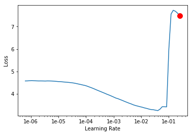
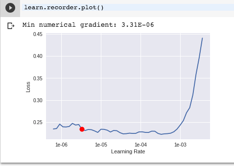
The goal with spline fitting is to overcome the problems with np.gradient when lr vs loss plot is very shaky. In terms of implementation, I don’t think directly fitting spline on smoothed loss is a problem, since we are trying to find the acceptable and large learning rates on the smoothed plot rather than mistaken outliers. But, still there is no guarantee this method will cover all the edge cases.
Yes, this (shakyness) is the very reason which motivated the implementation of a moving average. But the moving average retards the plot, so I was thinking about viable alternatives.
I found this problem quite interesting. Anyone know any existing guide on how to eye-ball these graph, with a variety of samples? I am aware these are discussed in the lesson, but it isn’t always easy to find.
I also thought the initial proposal is interesting. I am not sure if it can largely be automated. i.e. have lr_find(…) output the graph and then just search lr with multiple runs with cycles (tuning it like good old days), and empirically select the “best” lr. Thus, you can have a collection of X, Y pair to train the regression model? Do this for a large variety of models and dataset. I know this is expensive computationally, and may well be a research project. But then the “side effect” is you really know if L. Smith is largely right or wrong empirically. i.e. the proposal that the “near optimal LR” can entirely by gleaned from a plot of loss vs. the running lr.
I may well be underestimating something here…
Update: If i interprets right, L Smith never really emphasize on this, he just may have stated it as a heuristics for finding the upper bound for LR. He seemed to have used non-Hessian 2nd derivatives related method to do so in his other paper. I guess he wouldn’t care.
Also I saw there’s a PR where the spline method is used. I think this one is interesting. If it’s done over the EMA, then there will be a lag. Nevertheless, if the estimated LR is a good one, then we can just do a search around this point, and empirically determine the best LR. This may help speed up generating training pairs.
Additional thinking on the ML/DL approach.
I thought a RNN may be an alternative model than CNN. I don’t have experience with converting a time series to an image. Would the image be sensitive to the x, y scale or other visual feature. I think a combination of RNN and 1-D CNN may be a better approach.
I mean if you have CGPU to spare, combine all 3 as ensembles.
I am not sure if a paper with approx title “Learning to learn” is related to this thread. I will take a look at that paper when i get chance.
Thats a good point. EMA has a lag. I haven’t gone through code detail. This gets worse the more you smooth. Another concern is if the EMA has any “bias correction” or not. Else, the estimate will be even worse for earlier LR. This means if you fit a spline on it, the whole shape may or may not get influenced noticeably by this.
However, not sure if a spline over the raw data look?
I think this feature will be interesting to try out to see if it works better than eye balls.
Here is another gem (lr_find on unet):

looks like snakes and apples to me. and it’s not going to make it.
Is the red dot a location where dL/dLR has the steepest negative sloop? is that the heuristic to find the LR for eye ball?
I think this is adding up evidence we should do this by deep learning. This sort of thing just reminded me of “technical analysis” in stock mkt.
Random question about the autolrfinder.
Could we try to find out all the peak/local maxima of the time series. draw squares around it, find the"biggest" square. Within this square find how far is the local minima and go X% before it.
This assume that the biggest square is where you actually have the lr you care about.
So for example if your square is delimited by x1<x2 and the local minima xl is like this x1<xl<x2 then you can calculate the lr by doing something like xl - (x2-xl)*coef where coef is something you define.
Does this makes sense?
Maybe draw some sketches to go with your explanation.
I am not sure if all such rules/heuristic maybe fragile, if @stas keeps finding cases that will break. If our eye balls perform better, i would still advocate the original proposal of this thread, use a DL model to help another DL model.
Is this feature already in the master?

It printed out min numeric gradient and a red dot. I surly don’t want that to be my max_lr ?
Also, i assume this should be documented on how the red dot is computed, so if someone can kindly point out where I can read. I am aware it may be in this thread, but it is a long winded discussion.
Seems like that’s more an issue with the bounds than it is with the finder. It’s including data well after the explosion of loss.
My collaborator Angela (@cnll0075) and I are doing an ablation right now and using something not far from this to come up with a representation of learning rate that relates it to the maximum slope and what we call the elbow or the point of divergence. Rather than take @jeremy / @sgugger 's word on the best spot being approximately near the max slope we’re exploring where along the slope works best in the hopes that we can come up with some guidelines, althought it’s still early.
Here’s what we capture for every run:
- Maximim negative slope lr
- Minimum loss lr
- Elbow point lr (the point where loss explodes)
- mean slope between max and elbow
- stdev of slope between max and elbow
The latter two are there to help us try to charactarize the shape of the loss slope, namely are we doing a transfer and the slope looks different, but we also figure that it may prove useful in coming up with an automatic loss that is a bit more sophisicated that just ‘pick the max slope’. There are probably some other representations that would be useful to help charactarize the slope, and we’d love suggestions of other ways to charactarize the slope that we could use in hyperparameter selection but this is what we started with.
When selecting lr as a hyperparameter we limited our range to two different sets depending on the experiment:
- [max negative slope lr / 10 : elbow]
- [max negative slope lr / 10 : max negative slope lr * 10]
using an exponential scale for selection. We also experimented a little with using the selected value / 10 when transfer learning as we found selecting it independently was often clobbering good early results.
We’re running a number of experiments, but hopefully will have something to post here in the next few months. Definitely interested in hearing about what others are capturing / doing here and we’re open to input.
I am removing the suggestion as being the default behavior since it’s still very wacky (pass suggestion=True to get it back).
Spoke with Jeremy and in his experiments with platform.ai they found that:
- max -ve grad on smoothed grads works ok
- but 10x lower than minimum (moving avg of losses) loss works better (he admits it, finally
 )
)
I’d suggest to tweak the suggestion to show both those options, and when we see it work properly it can become the default behavior again.
So you are saying the recommendation as of now is to set the max LR to the elbow / 10?
Min loss isn’t always at the elbow.
@sgugger Do you find that it works for transfer learning as well? Annecdotally speaking, I often find the min loss lr to be quite low sometimes, and you can usually get away with setting it at the min closest to the elbow.
For transfer learning, you can go closer to the point of divergence yes (which isn’t the minimum). Again, the LR Finder is mostly there to give you the general order of magnitude, not necessarily the perfect value.
For sure, just wanted to confirm with you in the context of an auto-lr finder given your experience exploring this space.
I am still skeptical an auto-lrfinder can really work, but happy to be proved wrong  .
.
I still struggle to understand the general setting which led you to implement the LR finder the way it was (mind that I’m not criticizing), that is, set all the learning rates while being led just by the feedback from the fully connected group.
For example: the LR finder just plots the last layer group. Now, imagine a situation in which the training led the earlier layers to be already perfectly tuned, as opposed to the last convolutional and/or the FCs which still need training. While we use the LRF, we cannot have any clue of such an eventuality, but if the LRF could plot all the layer groups, one could freeze what should be frozen (or at least reduce the LR), and more generally set the appropriate LRs for every layer group.
This paper discussion might be of interest to the group:
There was a method described whereby you can examine the generalization of a given layer with a pretty simple implementation. There’s a chance it could be used here as well to tell whether the layers need more or less lr.
One thing I noticed after recently implementing a net and running it with the same hyperparameters over and over to get a sense of it’s variance is that the lr finder plots can vary significantly from network to network. Something to consider when building a tool that automates finding the learning rate.