Unofficial Lecture 9 Notes
Hi all, apologize for the delay, here’s the lecture 9 notes
Tim
import sys
sys.path.append('/Users/tlee010/Desktop/github_repos/fastai/')
%reload_ext autoreload
%autoreload 2
%matplotlib inline

from fastai.nlp import *
from sklearn.linear_model import LogisticRegression
# from torchtext import vocab, data, datasets
from fastai.io import *
path = './'
FILENAME='mnist.pkl.gz'

def load_mnist(filename):
    return pickle.load(gzip.open(filename, 'rb'), encoding='latin-1')

((x, y), (x_valid, y_valid), _) = load_mnist(path+FILENAME)
mean = x.mean()
std = x.std()
x=(x-mean)/std
mean, std, x.mean(), x.std()
x_valid = (x_valid-mean)/std
x_valid.mean(), x_valid.std()
(-0.0058509219, 0.99243325)
md = ImageClassifierData.from_arrays(path, (x,y), (x_valid, y_valid))
if you are missing the en library
#!python -m spacy download en
Auto Encoder
When you have unlabeled data. How can you create a NN that makes a features for you if you dont have the dependent variable. Lets have our input be the output as well.
Reconstruct the details of this insurance policy.
Less activations than inputs. Will compress features down into fewer features and then expand it back out. Great way for making embeddings and features even when you don’t have labels
Denoising the Auto Encoder
Start with a noisy version and then come out with the clean dataset. The 15% were randomly replaced with another row. The dependent variable would stay the same. Can show a lot of different rows. Gave him features (first layer weights), then took the NN and trained it on the claims data.
2 Models would have been enough to win.
He did no feature engineering
Embeddings
From last week
Iterators & Streaming
Its a object that we call next on. We can pull different pieces, ordered or randomized that can be pulled for mini-batches.

Pytorch is designed to handle this concept too, of predicting a stream of data (or the next item). fastai is also designed around this concept of iterators. DataLoader is created with the same concept, but with multiprocessing, which is multi threaded applications ( so you can use your entire processor)
Variable - keeps track of computations being made to a tensor. It’s a wrapper
pytorch - autograd
http://pytorch.org/docs/master/autograd.html
If we call back it will calculate the gradient.
def get_weights(*dims): return nn.Parameter(torch.randn(*dims)/dims[0])

class LogReg(nn.Module):

    def __init__(self):
        super().__init__()
        self.l1_w = get_weights(28*28, 10)  # Layer 1 weights
        self.l1_b = get_weights(10)         # Layer 1 bias

    def forward(self, x):
        x = x.view(x.size(0), -1)
        x = torch.matmul(x, self.l1_w) + self.l1_b  # Linear Layer
        x = torch.log(torch.exp(x)/(1 + torch.exp(x).sum(dim=0)))        # Non-linear (LogSoftmax) Layer
        return x
def score(x, y):
    y_pred = to_np(net2.forward(Variable(x)))#.cuda())))
    return np.sum(y_pred.argmax(axis=1) == to_np(y))/len(y_pred)
A re-write of fit
net2 = LogReg()#.cuda()
loss=nn.NLLLoss()
learning_rate = 1e-3
optimizer=optim.Adam(net2.parameters(), lr=learning_rate)

for epoch in range(1):
    losses=[]
    dl = iter(md.trn_dl)
    for t in range(len(dl)):
        # Forward pass: compute predicted y by passing x to the model.
        xt, yt = next(dl)
        y_pred = net2.forward(Variable(xt))#.cuda())

        # Compute and print loss.
        l = loss(y_pred, Variable(yt))#.cuda())
        losses.append(l)

        # Before the backward pass, use the optimizer object to zero all of the
        # gradients for the variables it will update (which are the learnable weights
        # of the model)
        optimizer.zero_grad()

        # Backward pass: compute gradient of the loss with respect to model
        # parameters
        l.backward()
        # print(loss.data)

        # Calling the step function on an Optimizer makes an update to its
        # parameters
        optimizer.step()

    val_dl = iter(md.val_dl)
    val_scores = [score(*next(val_dl)) for i in range(len(val_dl))]
    print(np.mean(val_scores))
0.910429936306
Within a fit lets rewrite some of the functions (gradient and step)
optimizer.zero_grad()

optimizer.step()
This code will be replaced with the following:
        if w.grad is not None:
            w.grad.data.zero_()
            b.grad.data.zero_()

        # Backward pass: compute gradient of the loss with respect to model parameters
        l.backward()
        w.data -= w.grad.data * lr
        b.data -= b.grad.data * lr
All gradients have to be added together to get that gradient for that parameter.
-
wis the variable we set before -
.gradreferring to the gradient part of the variable -
.data.zero_will zero the gradients, note this is the initializing
w.grad.data.zero_()
net2 = LogReg()#.cuda()
loss_fn=nn.NLLLoss()
lr = 1e-2
w,b = net2.l1_w,net2.l1_b

for epoch in range(1):
    losses=[]
    dl = iter(md.trn_dl)
    for t in range(len(dl)):
        # Forward pass: compute predicted y by passing x to the model.
        xt, yt = next(dl)
        y_pred = net2.forward(Variable(xt))#.cuda())

        # Compute and print loss.
        l = loss(y_pred, Variable(yt))#.cuda())
        losses.append(loss)

        # Before the backward pass, zero the gradients for all of the parameters
        if w.grad is not None:
            w.grad.data.zero_()
            b.grad.data.zero_()

        # Backward pass: compute gradient of the loss with respect to model parameters
        l.backward()
        w.data -= w.grad.data * lr
        b.data -= b.grad.data * lr

    val_dl = iter(md.val_dl)
    val_scores = [score(*next(val_dl)) for i in range(len(val_dl))]
    print(np.mean(val_scores))
0.905155254777
Going backwards
Momentum fastai can speed up the iteration rate and looping.
-
optimizer.step()- updates -
optimizer.zero_grad()- -
fit- is the loop that cycles through -
nn.Softmax- does the softmax calculation -
nn.Linear- does the linear multiplication
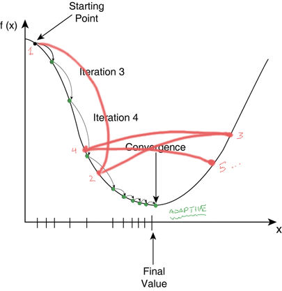
A word on learning rate
Sometimes if your learning rate is too large, it gets hard to converge near the later iterations
will pull out the parameters of the model
How many weights vs. the size of the data. Since our dataset is small, and our weights are very large, chances are that we will dramatically overfit.
t = [ 0.numel() for o in net.parameters]
t, sum(t)
  File "<ipython-input-25-112692b70a57>", line 1
    t = [ 0.numel() for o in net2.parameters]
                ^
SyntaxError: invalid syntax
Regularization
Add new terms to the loss function. If we add L1 and L2 norms of the weights to the loss functions, it incentives the coefficients to be zlose to zero. See the extra term below.
$$ loss =\frac{1}{n} \sum{(wX-y)^2} + \alpha \sum{w^2} $$
How to implement?
- Change the loss function
- Change the training loop to add the derivative adjustment <-- weight decay (not the same as momentum)
net = nn.Sequential(
    nn.Linear(28*28, 100),
    nn.ReLU(),
    nn.Linear(100, 10),
    nn.LogSoftmax()
)
loss=nn.NLLLoss()
metrics=[accuracy]
opt=optim.SGD(net.parameters(), 1e-1, momentum=0.9)
fit(net, md, epochs=5, crit=loss, opt=opt, metrics=metrics)
Failed to display Jupyter Widget of type HBox.
If you're reading this message in the Jupyter Notebook or JupyterLab Notebook, it may mean that the widgets JavaScript is still loading. If this message persists, it likely means that the widgets JavaScript library is either not installed or not enabled. See the Jupyter Widgets Documentation for setup instructions.
If you're reading this message in another frontend (for example, a static rendering on GitHub or NBViewer), it may mean that your frontend doesn't currently support widgets.
[ 0.       0.33271  0.28169  0.92725]
[ 1.       0.22736  0.24474  0.94715]
[ 2.       0.23459  0.26795  0.94118]
[ 3.       0.21125  0.27423  0.94805]
[ 4.       0.21197  0.32224  0.9384 ]
opt=optim.SGD(net.parameters(), 1e-1, momentum=0.9, weight_decay=0.3)
fit(net, md, epochs=5, crit=loss, opt=opt, metrics=metrics)
Failed to display Jupyter Widget of type HBox.
If you're reading this message in the Jupyter Notebook or JupyterLab Notebook, it may mean that the widgets JavaScript is still loading. If this message persists, it likely means that the widgets JavaScript library is either not installed or not enabled. See the Jupyter Widgets Documentation for setup instructions.
If you're reading this message in another frontend (for example, a static rendering on GitHub or NBViewer), it may mean that your frontend doesn't currently support widgets.
[ 0.       1.11321  1.13041  0.62271]
[ 1.       1.08937  1.06073  0.70482]
[ 2.       1.04438  1.35849  0.46795]
[ 3.       1.08236  1.12079  0.63515]
[ 4.       1.08296  1.20425  0.62988]
On to NLP!
!wget http://ai.stanford.edu/~amaas/data/sentiment/aclImdb_v1.tar.gz
--2017-11-30 14:16:02-- http://ai.stanford.edu/~amaas/data/sentiment/aclImdb_v1.tar.gz
Resolving ai.stanford.edu... 171.64.68.10
Connecting to ai.stanford.edu|171.64.68.10|:80... connected.
HTTP request sent, awaiting response... 200 OK
Length: 84125825 (80M) [application/x-gzip]
Saving to: âaclImdb_v1.tar.gzâ
aclImdb_v1.tar.gz 100%[===================>] 80.23M 10.6MB/s in 10s
2017-11-30 14:16:12 (7.80 MB/s) - âaclImdb_v1.tar.gzâ saved [84125825/84125825]
!gunzip aclImdb_v1.tar.gz
#!tar -xvf aclImdb_v1.tar
PATH='aclImdb/'
names = ['neg','pos']
trn,trn_y = texts_from_folders(f'{PATH}train',names)
val,val_y = texts_from_folders(f'{PATH}test',names)
def texts_from_folders(src, names):
    texts,labels = [],[]
    for idx,name in enumerate(names):
        path = os.path.join(src, name)
        for fname in sorted(os.listdir(path)):
            fpath = os.path.join(path, fname)
            texts.append(open(fpath).read())
            labels.append(idx)
    return texts,np.array(labels)
??texts_from_folders
trn[0]
"Story of a man who has unnatural feelings for a pig. Starts out with a opening scene that is a terrific example of absurd comedy. A formal orchestra audience is turned into an insane, violent mob by the crazy chantings of it's singers. Unfortunately it stays absurd the WHOLE time with no general narrative eventually making it just too off putting. Even those from the era should be turned off. The cryptic dialogue would make Shakespeare seem easy to a third grader. On a technical level it's better than you might think with some good cinematography by future great Vilmos Zsigmond. Future stars Sally Kirkland and Frederic Forrest can be seen briefly."
First we will throw away the order of words --> Bag of words
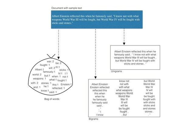
Let’s use sklearn to convert corpus to bag of words
veczr = CountVectorizer(tokenizer=tokenize)
Key Concepts
Vocabulary - need to find the unique terms throughout the entire corpus
Term Document Matrix
- columns - vocab or words
- rows - different documents
- cells - count of occurance
Sentiment Approach: bays rule
The probability that a document is from class 1 given that the document is from class 0. We will use a conditional probability as follows below
$$ \frac{P(C_1 | d)}{P(C_0 | d}) = \frac {P(d|C_1)P(C_1)}{P(d)} = \frac {P(d|C_1)P(C_1)}{P(d|C_0)P(C_0)}$$
How do we calculate?
- Gather the documents of one class together
- Create profile made up of the words, and their probabilities
- Note: we add a dataset that assumes every word occurs at least one in the document
- We should have a probability per word, for each class
- For each doucment we can multiple the coefficients and that will give us a P(C_1 | d) and P(C_0 | d)
we will learn the word features from the training set and split. Then use the same framework to split the test set
trn_term_doc = veczr.fit_transform(trn)
val_term_doc = veczr.transform(val)
We now have 25000 words, with 75132 docs
trn_term_doc
<25000x75132 sparse matrix of type '<class 'numpy.int64'>'
	with 3749745 stored elements in Compressed Sparse Row format>
Sparse Matrix
Special format when most of your matrix is filled with zeros. This assumes that most of the matrix is zero, and only keep track of the elements that are non-zero.
The first feature has 93 items
trn_term_doc[0]
<1x75132 sparse matrix of type '<class 'numpy.int64'>'
	with 93 stored elements in Compressed Sparse Row format>
What are the features (words) ?
vocab = veczr.get_feature_names(); vocab[5000:5005]
['aussie', 'aussies', 'austen', 'austeniana', 'austens']
Lets look at our 93 words
w0 = set([o.lower() for o in trn[0].split(' ')]); #w0
Look up a specific word
veczr.vocabulary_['absurd']
1297
How many times does this word show up in document 1
trn_term_doc[0,1297]
trn_term_doc[0,5000]
Naive Bayes
We define the log-count ratio r for each word f:
$r = \log \frac{\text{ratio of feature f in positive documents}}{\text{ratio of feature f in negative documents}}$
where ratio of feature f in positive documents is the number of times a positive document has a feature divided by the number of positive documents.
p = x[y==1].sum(0)+1 - Number of times it shows in positive corpus
p = x[y==0].sum(0)+1 - Number of times it shows in negative corpus
r = np.log((p/p.sum())/(q/q.sum())) - summing logs is a lot easier to do, otherwise you might run into float errors
b = np.log(len(p)/len(q)) - this is our naive bays
x=trn_term_doc
y=trn_y

p = x[y==1].sum(0)+1
q = x[y==0].sum(0)+1
r = np.log((p/p.sum())/(q/q.sum()))
b = np.log(len(p)/len(q))
Here’s our predictions from Naive Bayes ~ 80% positive
pre_preds = val_term_doc @ r.T + b
preds = pre_preds.T>0
(preds==val_y).mean()
0.80740000000000001
Binarized: instead of using the 0.66 for a word, why not just 1 if the word shows up. 83% chance
pre_preds = val_term_doc.sign() @ r.T + b
preds = pre_preds.T>0
(preds==val_y).mean()
0.82623999999999997
Logistic Regression
Here is how we can fit logistic regression where the features are the unigrams. So instead of using bayes, we set it up like a supervised problem
m = LogisticRegression(C=1e8, dual=True)
m.fit(x, y)
preds = m.predict(val_term_doc)
(preds==val_y).mean()
0.85648000000000002
Regularized version -> 0.0000001
m = LogisticRegression(C=1e8, dual=True)
m.fit(trn_term_doc.sign(), y)
preds = m.predict(val_term_doc.sign())
(preds==val_y).mean()
0.85528000000000004
Regularized version -> 0.1
m = LogisticRegression(C=0.1, dual=True)
m.fit(x, y)
preds = m.predict(val_term_doc)
(preds==val_y).mean()
0.88271999999999995
Regularized version -> 0.1 with traing doc terms
m = LogisticRegression(C=0.1, dual=True)
m.fit(trn_term_doc.sign(), y)
preds = m.predict(val_term_doc.sign())
(preds==val_y).mean()
0.88404000000000005
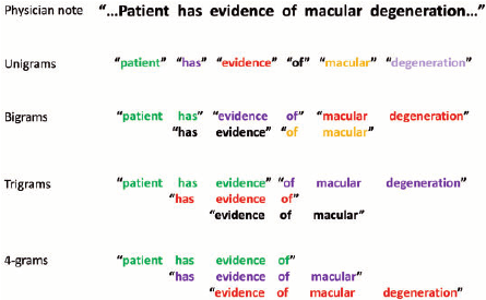
Trigram with NB features
Instead of using words, we will use small phrases of words, or phrases. In this case we will use 3 word phrases, also referred to as trigrams
veczr =  CountVectorizer(ngram_range=(1,3), tokenizer=tokenize, max_features=800000)
trn_term_doc = veczr.fit_transform(trn)
val_term_doc = veczr.transform(val)
Let regularization do the feature selection, just bound the overall space
trn_term_doc.shape
(25000, 800000)
vocab = veczr.get_feature_names()
vocab[200000:200005]
['by vast', 'by vengeance', 'by vengeance .', 'by vera', 'by vera miles']
y=trn_y
x=trn_term_doc.sign()
val_x = val_term_doc.sign()
p = x[y==1].sum(0)+1
q = x[y==0].sum(0)+1
r = np.log((p/p.sum())/(q/q.sum()))
b = np.log(len(p)/len(q))