This is an interesting experiment conducted by a fellow under fast.ai’s International Fellowship 2018 that dig into Leslie Smith’s work that Leslie describes the super-convergence phenomenon in this paper, “A Disciplined Approach to Neural Network Hyper-Parameters: Part 1 - Learning Rate, Batch Size, Momentum, and Weight Decay”.
Results from the experiments:
By training with high learning rates we can reach a model that gets 93% accuracy in 70 epochs which is less than 7k iterations (as opposed to the 64k iterations which made roughly 360 epochs in the original paper).
This cyclical learning rate and momentums notebook contains all the experiments.
IMO, I think it’s too early to tell how well this technique works in general until we do more work to evaluate this. Nevertheless, I think this is an interesting and promising technique.
Note: everything that follows is unofficial.
The bleeding edge version (beta) of fastai library supports this technique. We can try it out by doing a git pull from fastai repo. Next is a high level summary of fastai library changes for this feature and some quick documentations:
1. New cyclical momentum
To use, add use_clr_beta parameter in the fit function that controls the 1cycle policy. For example:
learn.fit(0.8, 1, cycle_len=95, use_clr_beta=(10, 13.68, 0.95, 0.85), wds=1e-4)
The arguments of the use_clr_beta=(div, pct, max_mom, min_mom) tuples mean:
div: the amount to divide the passed learning rate to get the minimum learning rate. E.g.: pick 1/10th of the maximum learning rate for the minimum learning rate.pct: the part of the cycle (in percent) that will be devoted to the LR annealing after the triangular cycle. E.g.: dedicate 13.68% of the cycle to the annealing at the end (that’s 13 epochs over 95).max_mom: maximum momentum. E.g.: 0.95.min_mom: minimum momentum. E.g.: 0.85.
Note, the two last args can be skipped if you don’t want to use cyclical momentum.
2. New learning rate finder function, lr_find2
This is a variant of lr_find. It doesn’t do an epoch but a fixed number of iterations (which may be more or less than an epoch depending on your data). At each step, it computes the validation loss and the metrics on the next batch in the training loop for the next batch of the validation data, so it’s slower than lr_find.
An example from the notebook under “Tuning weight decay” section:
learn.lr_find2(wds=1e-2, start_lr=0.01, end_lr=100, num_it=100)
The arguments of lr_find2(start_lr, end_lr, num_it, wds, linear, stop_dv)
start_lr: learning rate(s) for a learner’s layer_groups.end_lr: the maximum learning rate to try.num_it: the number of iterations you want it to run weight decays,wds.stop_dv: stops (or not) when the losses starts to explode.
3. New plots
With lr_find2(), validation losses and metrics are saved each time they are computed (whether in normal training or LR find) so we can plot them after if we want.

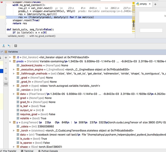
 at least it shows the culprit is really the variable y