I am also having that problem. I think the point of watching on course.fast.ai is just so we can find things like the wiki, but obviously you already found all the resources  So I think you’re good-- watch it on YouTube, but post your questions here, not in the YouTube comments. I don’t think there is any difference in the video content, since the one that is normally on course.fast.ai is just linked to YT.
I’m having an issue with running the rossmann example.
Step 8: for t in tables: display(DataFrameSummary(t).summary())
I am running into an issue with pandas.
It’s telling me:
module ‘pandas.core.common’ has no attribute ‘is_numeric_dtype’
Any ideas on how to fix this?
1 Like
Hi, I also encountered the same issue and I googled a bit.
At this time, the easiest solution is to skip the cell because the cell just displays the summaries of dataframes and does not manipulate any element in datarames.
The issue is from the pandas_summary library.
It calls pandas is_numeric_dtype method though, the location of the method is changed now. This is why the error occurs.
1 Like
Heya D,
I ran into the same issue but continuing on with the notebook I couldn’t see that it affected anything. The remainder of the lesson ran fine (although when i tried it a few days ago it was getting hung up on the tables, i do Git Pull and Conda Env Update pretty often so that might have helped).
1 Like
I’m going to try and move to the FastAI AMI and not use sagemaker prebuilt image as I am wondering if that’s my issue.
The issue is a new Pandas library was released in early May, version 23 and it has a bug for the DataFrameSummary.
I was able to resolve the issue by going back to pandas version 22 by using the command
conda install pandas=0.22
1 Like
you can also use for t in tables: print(t.describe())
it will show the same data, just not in a html table
1 Like
exp_rmspe : metrics vs explicit calculation.
I was able to run through the whole rossman notebook. I also created my copy from scratch to make sure I fully understand. Overall, I am pretty familiar with the idea and code base behind the scene now.
But I got a small questions regarding the result. See the following lines from the notebook:
m.fit(lr, 2, metrics=[exp_rmspe], cycle_len=4)
# m.save('awang_val0')
# m.load('awang_val0')
x,y=m.predict_with_targs()
len(x), len(y), exp_rmspe(x,y)
For the first line, I got the following output:
epoch trn_loss val_loss exp_rmspe
0 0.007935 0.012073 0.108804
1 0.006928 0.010902 0.09866
2 0.00581 0.010534 0.09842
3 0.005843 0.010511 0.097418
4 0.007132 0.011242 0.10067
5 0.007127 0.011706 0.100811
6 0.005701 0.010629 0.097536
7 0.005325 0.010472 0.097566
For the last line, I got:
(38399, 38399, 0.10119025162931043)
From last epoc of fit() to m.predict_with_targs(), nothing changed to the learner m. I checked the code, both exp_rmspe were calculated on validation set. Shouldn’t they be the same?
For the validation set, I used:
val_idx = np.flatnonzero((df.index<=datetime.datetime(2014,9,17)) & (df.index>=datetime.datetime(2014,8,1)))
If I use the original one:
val_idx=[0]
Then they matched.
It seems the exp_rmspe will return slightly different result for validation set if validation set is larger than one.
Do I miss anything?
I’m a little bit confused by matrix product on a fully connected layer on conv-example.xslx demonstration.
Jeremy says from approximately 1:09:10 to 1:09:23 that “a fully connected layer is doing classic traditional matrix product, basically just going through each pair in turn, multiplying them together and then adding them up to a matrix product”. But the formula in cell EN4 at 1:09:23 has in it a SUMPRODUCT() Excel function that does element-wise multiplication.
I thought it may have something to do with the fact that we have two matrices 12x13 on Maxpool layer, each multiplied by corresponding 12x13 matrices on Dense weights layer, and this can be seen as a 2x12x13 matrix multiplied by a 2x12x13 matrix, but traditional matrix product is only defined for two-dimensional matrices.
In short: Jeremy says it’s matrix product but I only see element-wise product. What did I miss?
@amir01, did you get an answer to your question? I have a related question.
I am doing the Planets competition, and initially trained my model using size 64 (created an ImageClassifierData object - one of its super classes’ object to be precise - with that size):
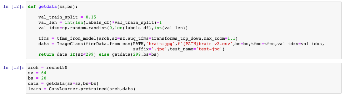
Then after training with Data Augmentation, I trained with differential rates and changing the size to 256. I check the value of the size variable of the data object, and get 64:
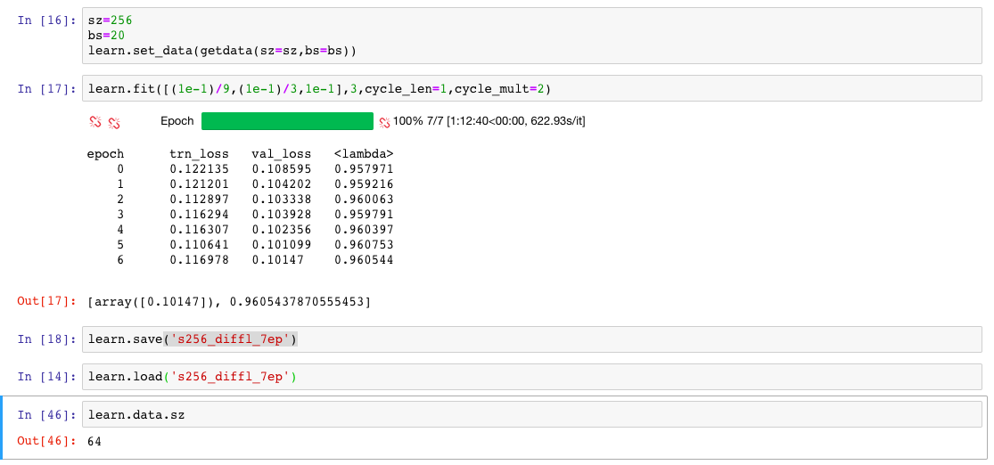
Isn’t it supposed to give 256 at this point?
Hope you can help. Thanks
@ekolodezeva I just assumed it was an error, because it didn’t make sense. Were you able to find out otherwise?
I dont know what you are doing but it is working fine in my case

try running all cells again and check if your fastai repo is updated
1 Like
No, I didn’t find out. I just assumed it was simply an error, as you say.
1 Like
Hi
Did you manage to do any progress with state farm? No matter what I do I’m completely stuck - either resnet50, resnext50 or resnext101.
I can’t get my model to achieve decent training/validation accuracy.
BTW - my earlier attempts included wrong validation set prep; i actually had the the same driver in both validation and training set, unlike to what kaggle asks; in those I achieved much better results (even on the test test) than what i achive now with proper validation separation - driver only shows in either test of validation stets.
I am doing Amazon Planet Space competition which Jeremy showed in lesson2-image_models.ipynb.
At the end of the notebook, learn.TTA() is called to get the log probabilities.
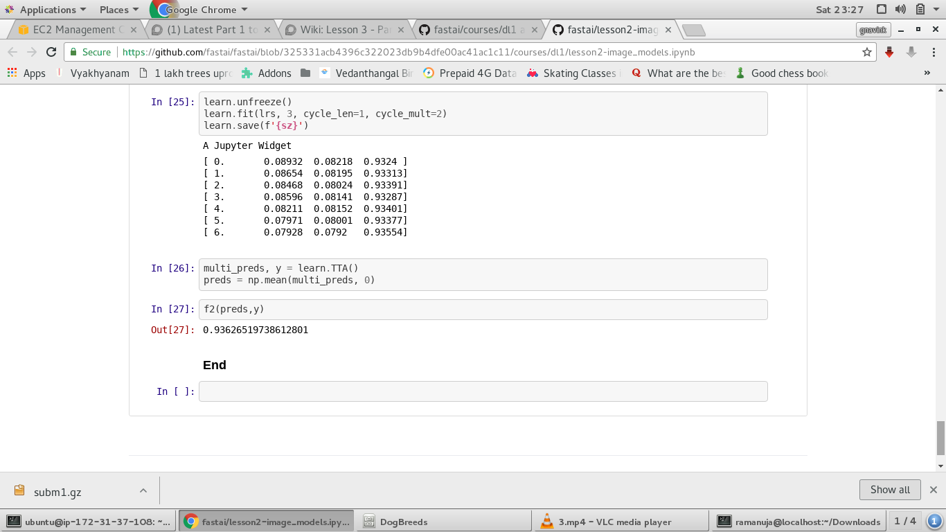
Unlike catsvs dogs / Dog breeds after doing learn.TTA() why the output from learn.TTA() is not converted to actual probabilities by calling np.exp() in this notebook.
I assume learn.TTA() always gives log_probabilities…
I printed the model both in Amazon Planet & DogBreeds.
The Amazon Planet is using sigmoid as the last activation layer, whereas
dog-breeds is using LogSoftMax as the last activation layer.
The below is the output from both my notebooks.
Planet Space Amazon Notebook: (lesson2-image_models.ipynb)
learn = ConvLearner.pretrained(f_model, data, metrics=metrics)
learn
(10): BatchNorm1d(1024, eps=1e-05, momentum=0.1, affine=True)
(11): Dropout(p=0.25)
(12): Linear(in_features=1024, out_features=512, bias=True)
(13): ReLU()
(14): BatchNorm1d(512, eps=1e-05, momentum=0.1, affine=True)
(15): Dropout(p=0.5)
(16): Linear(in_features=512, out_features=17, bias=True)
(17): Sigmoid()
Dog-Breeds Identification Challenge:
Sequential(
(0): BatchNorm1d(1024, eps=1e-05, momentum=0.1, affine=True)
(1): Dropout(p=0.25)
(2): Linear(in_features=1024, out_features=512, bias=True)
(3): ReLU()
(4): BatchNorm1d(512, eps=1e-05, momentum=0.1, affine=True)
(5): Dropout(p=0.5)
(6): Linear(in_features=512, out_features=120, bias=True)
(7): LogSoftmax()
)
Is that the reason why in the Amazon Planet Space notebook, the output from learn.TTA()
is not converted to probabilities using np.exp(). because its already in that form as given by sigmoid().
But whereas in dog-breeds its in log probabilities as returned by LogSoftmax() and hence converted to probabilities using np.exp()
Is my understanding correct?? Is the sigmoid() function defined by PyTorch ?
@jeremy you mentioned in the video that the Keras transfer learning example behaves strangely compared to the fast.ai/PyTorch version. I think the reason is that the Keras example doesn’t have an equivalent of bn_freeze.
Setting trainable = False on BN layers in Keras freezes the trainable parameters, but it doesn’t cause Keras to use the running mean/variance; it still uses the batch mean/variance. To fix this, you need to do
from keras import backend as K
...
K.set_learning_phase(0)
model = Model(inputs=base_model.input, outputs=predictions)
K.set_learning_phase(1)
Disabling the learning phase will cause Keras to use the running mean/var instead of the batch mean/var: https://github.com/keras-team/keras/blob/master/keras/layers/normalization.py#L202
The only other way would be to set training=False when calling the BN layer: https://github.com/keras-team/keras/blob/master/keras/layers/normalization.py#L130, but this only works if you modify the code for the base model.
Do you know why bn_freeze has such an impact on performance? I’ve been trying to retrain MobileNet, and it didn’t work at all until I used the Keras equivalent of bn_freeze. Without bn_freeze, Keras reports reasonable train and validation accuracy, but the accuracy plummets in testing.
I’m getting the following error, when I go to run the planet lesson 2 notebook:
data = get_data(256)
ParserError: Error tokenizing data. C error: Expected 1 fields in line 6, saw 2
I’m unsure what the issue is here… ?
Disregard. It was a corrupt file. Another download of the CSV fixed it.
It is crystally clear about the filters from input to Conv1: they are intended to detect top edges and side edges.
I might have missed in the video, but how are the filters from Conv1 to Conv2 were created? those
0.5 0.3 0.3
0.9 -0.5 0
0.8 0.01 -0.7
etc. Are they also parameters?