What should my learning rate be?

Thanks for the reply. I went with 0.001 based on my intuition. However, I am still quite not able to understand why would the loss increase and the decrease? Has it found a local minima?

Am I completely wrong in thinking that there is a relationship between learning rare finder and minimas?

I also see that sometimes. It’s very curious! I think that there are other “flat spots” it finds - for instance maybe setting “all zeros” or “all ones”.

3 Likes

@vikram

I hope not to say stuff which is trivial to you, I don’t know your background.

The error surface for a loss function is not only nonconvex, but also:

  1. Very bumpy

  2. Very high dimensional

The bumpiness does mean that if you select a very small learning rate (and/or a weak momentum), it won’t be able to jump out of shallow local minimum.

Its high dimensionality (millions of dimensions if you consider a model like vgg16, just to name one) does mean that you would almost certainly be wrong should you try to infer qualitative considerations using your intuition over an example 2d error surface immersed in 3d space.
The only tool which can provide reliable informations about such minima are the eigenvalues of the hessian. It is unpractical (and even infeasible) to routinely use such monster hessian (let alone doing its eigendecomposition) for deep learning, but you could try it if you want to gain a better qualitative understanding of an error surface relative to a small model.

More literate users will hopefully correct me if I’ve been inexact.

@jeremy

I didn’t understand what you exactly mean by saying: “[…] for instance maybe setting “all zeros” or “all ones”.

However, is there any documentation explaining how exactly your rate finder works?

It’s based on a paper …
Forgot the name but it’s like cyclic rates with cosine annealing and restarts…

Not completely sure

1 Like

Thanks, I think I found it, it’s Cyclical Learning Rates for Training Neural Networks by Leslie Smith.

Interesting.

The way this learning rate finder is implemented in fastai is simply as a learning rate scheduler that slightly increases the learning rate with every mini batch. It stops training when the loss suddenly becomes a lot higher.

When you get a plot like the above, I’m curious if you would also get a similar plot if the learning rate was not increased on every mini batch but only every 10 or so mini batches. Or what if you tried this with a larger batch size?

In other words, I’m wondering if it is the stochastic nature of the mini batches that is responsible for such a curve?

Source: an article by Carlos Perez. I saved the pic yesterday, but I don’t remember the page address. Search for the paper (and read it if possible) and you’ll find the article, too.

5 Likes

Nice! That does show things becoming smoother with a larger batch size (as is usually the case) but the curves still follow the same general shape. Only when the batch size becomes really small (8 or 4) is there an additional peak.

1 Like

You know what makes me feel a bit uneasy when studying deep learning? It’s like being a caveman experimenting with fire prior to any knowledge, even rudimentary about the physics of combustion. And this happens even in the academia.

Take Smith’s paper for example. It’s very interesting, and it shows useful experimental result. Still, it is pure experimentation at blind, indeed.

No theoretically grounded results are shown. No further insights about the topology of the loss surface are obtained

In their conclusions, the authors write:

Furthermore, we believe that a theoretical analysis would provide an improved understanding of these methods, which might lead to improvements in the algorithms.

That’s the way to go, in my opinion. Yet, I searched for them and found little or nothing, although something exists (also by Smith) about the forementioned topological insights (in a rather slacky sense, though).

I highlighted the parts I considered noteworthy:

smith II.pdf (551.3 KB)

1 Like

That is how pretty much all technological progress is made. Contrary to popular belief, the science comes after the engineering and the engineering is usually trial-and-error.

It would be great to have a better scientific understanding of how deep learning works, and academics are trying hard to come up with such theories, but in the end the only way to gather enough understanding to create such theories is by doing a lot of getting-your-hands-dirty experiments.

It’s a cyclical process: the engineering begets the science, which informs the engineering, which improves the science, and so on.

2 Likes

Good afternoon,

I ran the learning rate finder again after a few training epochs and the graph is shown as follows:

image

In the lessons, I understood that we choose the steepest point right before the flat point. Since there is no descending line, does this mean I can use any learning rate up to 0.01? Thank you in advance.

1 Like

It’s rather hard to interpret these graphs after training - based on this I’d try 1e-3 and 1e-2 and see what’s best.

1 Like

From my experience, if I tried various learning rates (and all other variations) and I still could not train the model properly. I will try different architectures and optimizers. I understand I don’t answer your question. But, it may be the way to move forward. It is part of the journey.

1 Like

Thank you for the link. I will have a good read :grinning:

1 Like

Just a side notes from online video lecture:
Learning rate is how fast model is learning that means how fast model is loosing the loss.
That’s why we need to choose learning rate at which point loss rate is high.
(Please correct it if it found wrong)

Mh, it would be so just in ideal conditions.
Let’s say that the learning rate is how big your jumps over loss surface are.

MY EXPLANATION
This are the explanations on what we learnt at course, part 1, lesson2 (18.40 in the video)

We put the graphs next to each other. And the idea is to minimize the loss function and to increase the LR.

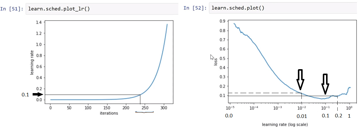
As we can see on the graph at left, there is a point on the iterations axis where the curve go dramatically up, exponentially. It is in a neighborhood of 250. This coresponds on the LR axis to the [0.0,0.2], more precisely to the [0.0,0.1] interval.
As we can see in the graph at right, the interval in discussion is 0.0=10**(-5) and 0.2 which is greater then 0.1=10**(-1). As the LR starts from 0=10**(-5) and increases with very small quantities, the loss function goes down steep enough. There is a point on LR axis in the graph at right where the loss function begins to go up. And we don’t want that. This is 10**(-1)=0.1. This the minimum. But we don’t want the point where the curve changes it’s shape and goes up, which means the increasing of loss, but instead a closer point, which is 10**(-2)=0.01. This is the point with the highest LR and the small loss.
This is the reason we chose 0.01 in the line of code learn.fit(0.01,3).

5 Likes

see my explanations looking the loss function and the learning rate.
codruta1968

see my explanations looking the loss function and the learning rate.
codruta1968