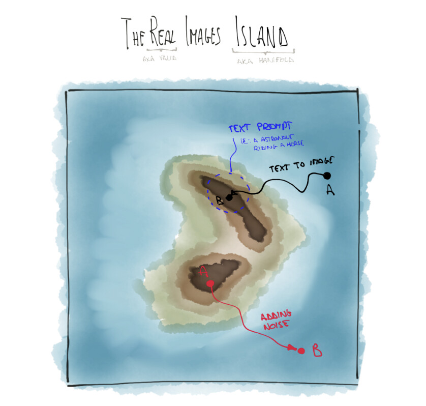
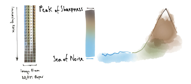
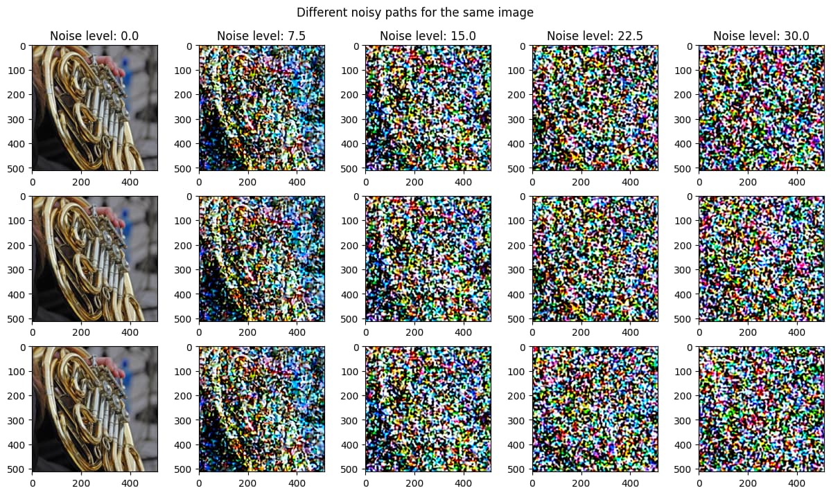
When I first came across some of the ideas behind stable diffusion, especially VAE and UNET with classifier-free guidance, I’ve pictured them in my mind like an island that has peaks of sharp images emerging from a big sea of pure noise.
VAE: is the (multi dimensional) space where we can move.
PROMPT: is the direction where we want to go.
UNET: is our “navigation system” that takes us out of the noise.
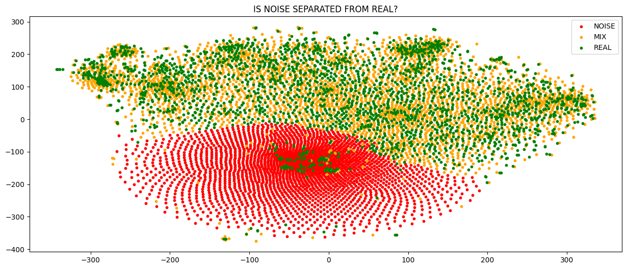
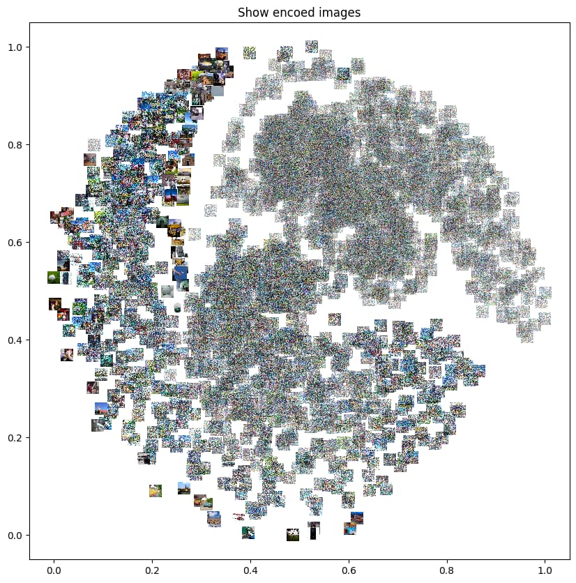
This notebook: searching_the_real_images_island.ipynb analyzes both VAE latents and UNET bottleneck latents using dimensionality reduction in order to understand if these techniques are able to highlight the concept of level of noise and lay out the data from the less noisy (peak of sharpness) to the most noisy one (sea of noise).
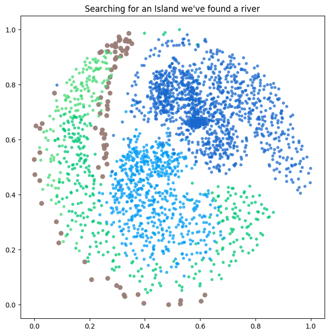
Finally after adding the UNET encode step to the latents a proper order arises and all the data seems now properly ordered by noise level.
…At the end of the day, I was searching for an island, but I’ve found a river
NOTE: code is not super optimized and to run end-to-end the notebook takes about 30 min and lot of gpu (I’ve run it on a 3090).
CREDITS: I want to thank @suvash, @strickvl and all the Delft study group for keeping me motivated on this. Finally a special thanks to @pcuenq for the support and the help with UNET encoder.
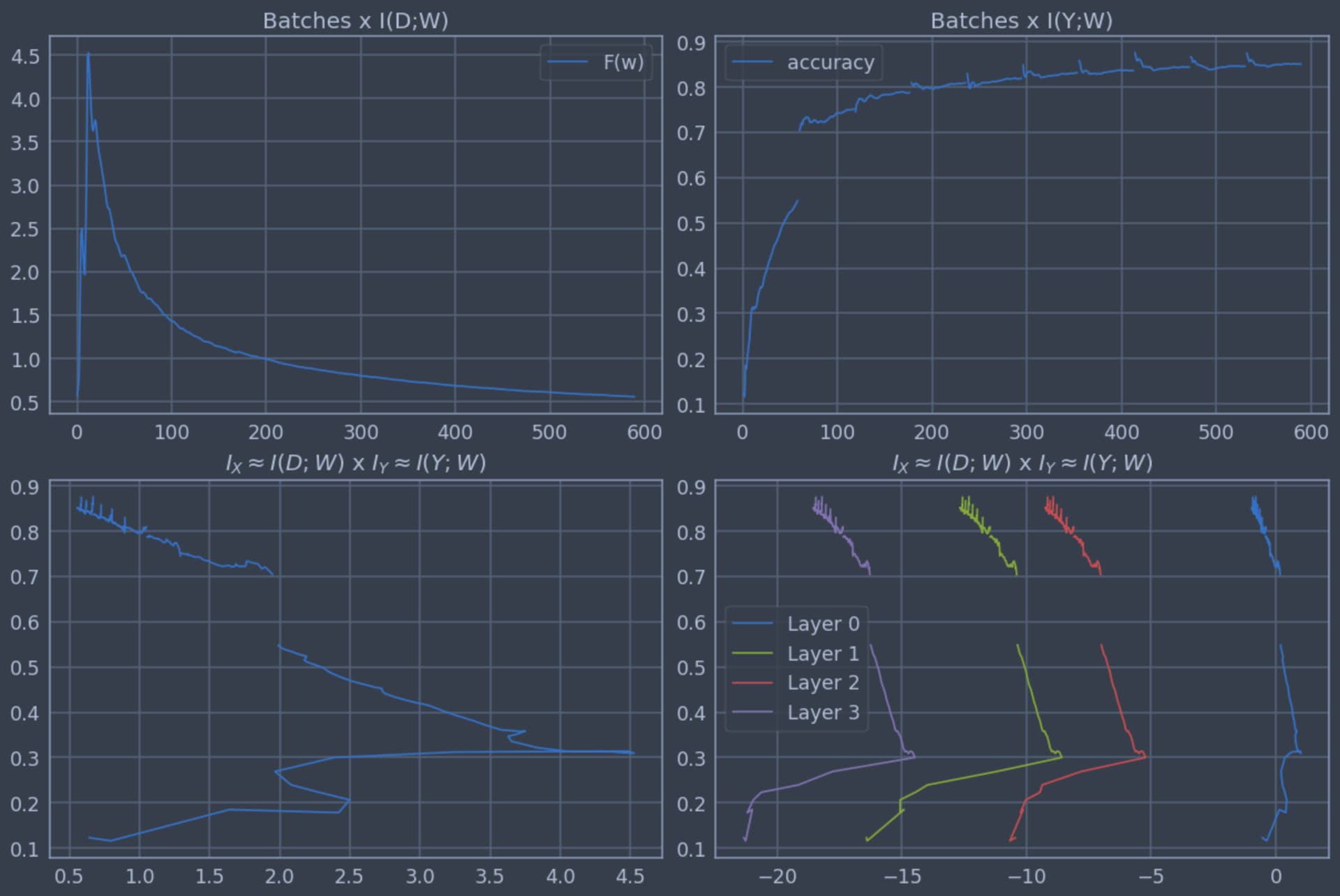
Most of the information in the dataset (D) is about the input data X, not the label Y. In the top left chart, we can see that the model quickly increase the information I(D;W), memorizing the dataset and increasing the accuracy (top right chart). During training, we expect the amount of information in the weights to decline, as observed in Batches x I(D;W).
In the bottom left chart (I_X \times I_Y), we relate the amount of information in the weights,which we assume is basically about X (I_X) with accuracy, which is a proxy for the information about the task (I_Y). The training starts at the bottom left of the chart and ends in the top left. We can see that most of the increase in accuracy happens while the model is forgetting information of X that is not relevant to the task Y.
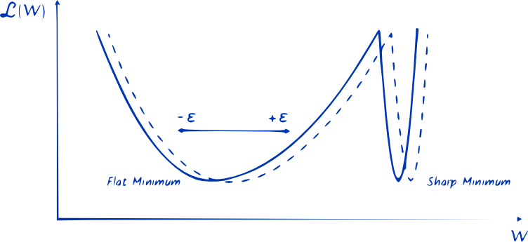
The less information in the weights, the flatter is the loss region of the minimum weights. Flat minima regions are preferred as a small change in the parameters do not imply a big change in the loss.
Another idea I had was to try to use the Fisher Information as an approximation for the Hessian of the loss. With that we can calculate the natural gradient. Unfortunately, my natural gradient optimizer did not outperform SGD yet. ¯_(ツ)_/¯
Great work Stefano, thanks for sharing. Some questions:
I may have missed something in your explaining of escape sequences. What I understood was that you vae_enconded a real image and then created a binary tree of noisy variations of the original latent. After 4 levels, you have original + 2 level1_noisy + 4… + 16 level4_noisy=31 latents. A escape sequence would be just a path in the binary tree. Is that right?
… but then you show a path in the unet_embedding space. It is not clear to me what you did here.
What is your opinion on why the unet embedding has a higher dimensionality than the inputs?
You talk about PCA but it then don’t use it. Is that right? Why?
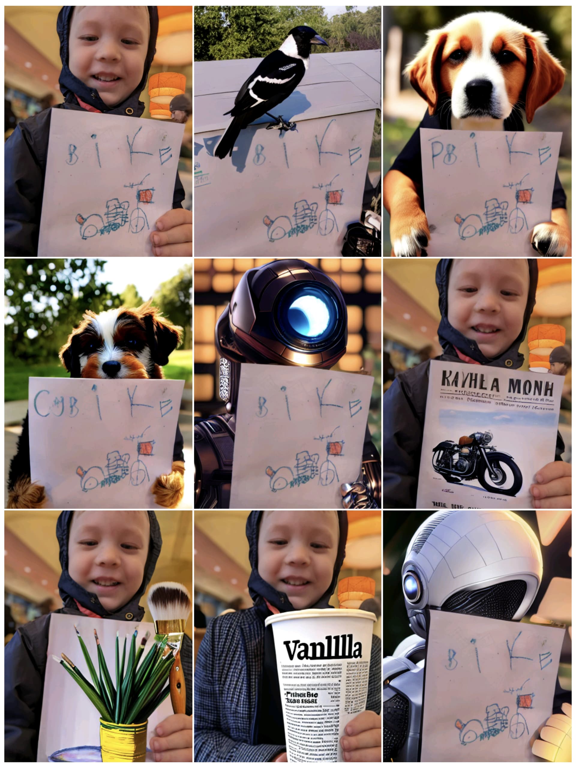
I really like how Conditioning Mask Strength is AWESOME! - AUTOMATIC1111 - YouTube hacks into the in-painting model to improve img2img where fun variations are introduced while still retaining source themes.I was able to reimplement this feature using Huggingface base modules on StabityAI/stable-diffusion-2-inpainting.
Yes: there are 31 variations that get “indexed” in 16 paths (so I don’t need to compute 16*16 variations). The path indexing array is noise_sequence_idxs (shape (16,5)) - each row is a “path” of 5 elements. The reason why I made this “noise schema” was to try to “imbalance” the problem towards noise - there are way more noise images than sharp one (aka: the sea is way bigger than land )
I tried to see if a on “unet space” samples are ordered in terms of noise level, and the fact that multiple paths from the same image shares lot of common nodes should help to define a “patch” of space with certain properties (I’m assuming/hoping that the unet embedding space is somehow continous).
That was a discovery! At first sight I thought that I made a mistake, but It seems that is really happening. BTW: have a bottleneck with higher dimensionality is something simular to what I’ve seen in other domains (ie: Stacked Hourglass Network); maybe this would probably help the signal to be transformed/integrated with the data learned by “encoder” and these new understandings will be used by decoder to properly get to the final result. … At the end of the day this seems to be a DECODER-ENCODER unet. maybe @johnowhitaker would have a better explanation.
When I want to reduce a high dimensionality signal I usually first use PCA to get rid of some dimensions and then use non linear methods for last steps, ie: [64*64*4 = 16k]-(PCA)->[1k]-(TSNE)->[2]
What I noticed here is that if you ask the PCA to “reduce dimensionality” of noisy samples (almost always, that’s weird!) it takes forever to compute; I’ve tried to play around with input parameters (ie: different svd_solvers), but with no luck, so I’ve disabled it. Given that PCA and SVD are strongly correlated, my intuition is that in pure noise there is no “pattern emerging”, so no approximate solution can avoid computing svd on a (sparse) enormous matrix: this is my explanation of why it takes so long to compute.
Although I’m behind on the class (lecture 16), I took some time to relax and play today (since it’s New Year’s Day where I am). Below are a few results from experiments with image Inpainting, and I wrote a blog post about the process and my impressions: https://www.alexejgossmann.com/stable-diffusion-inpainting/
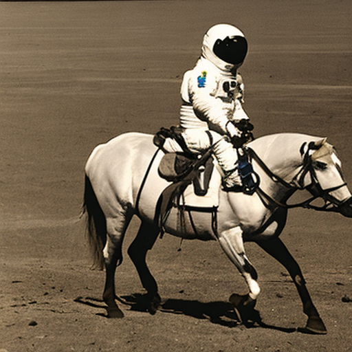
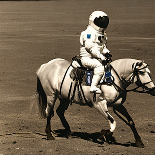
I recently made some experiments on Stable Diffusion’s sampling process, which I summarized in this blog post / notebook (thanks fastpages for making it so easy to publish notebooks as blog posts!!).
What I’ve done in a nutshell:
Analyzed how norms behave before and after guidance mechanism → the goal is to give intuition behind the “whole rescale” idea suggested by Jeremy
Some trajectory analysis/visualizations in the latent space (spoiler: weird things seem to happen, and I am not sure how to explain them)
In addition to the rescale mentioned above, 2 tuning methods for the sampling: 1/ prevent overshooting, which seems to create sharper images, but at the cost of noise, and 2/ polynomial trajectory regression, which seems to smooth the image at the cost of details in the image.
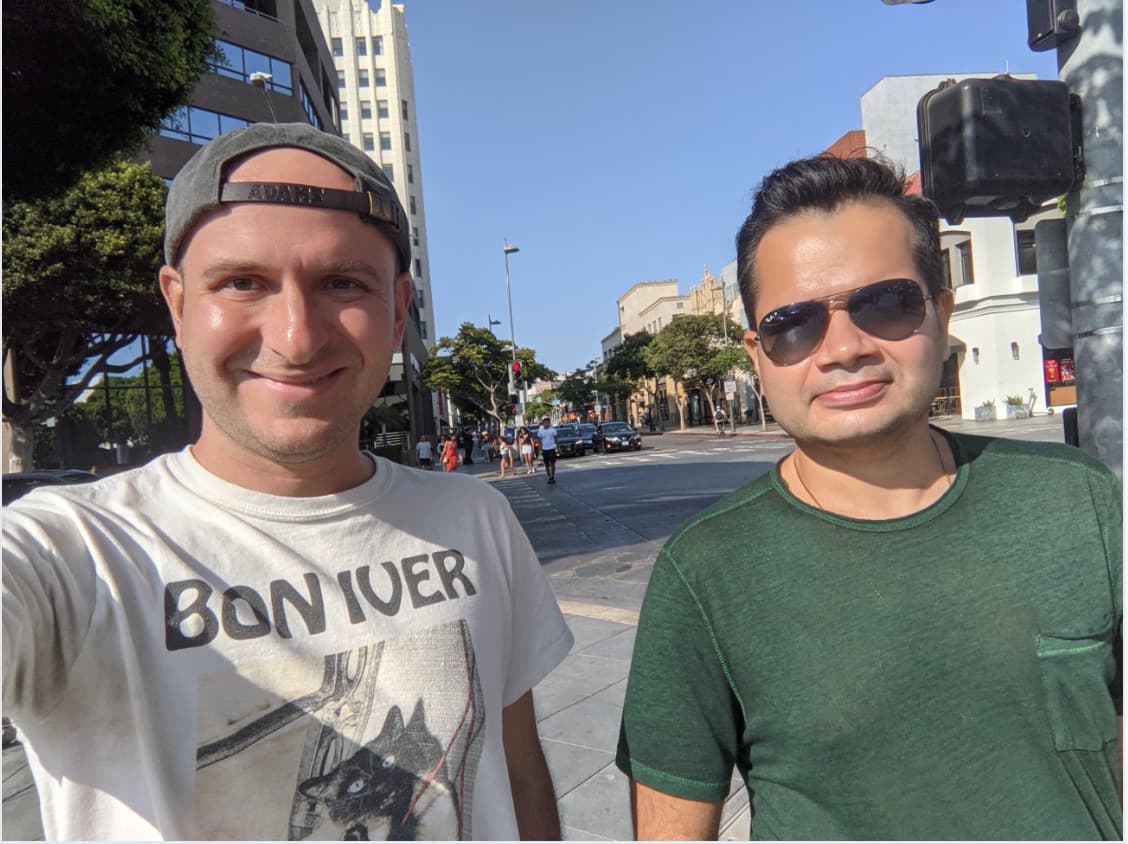
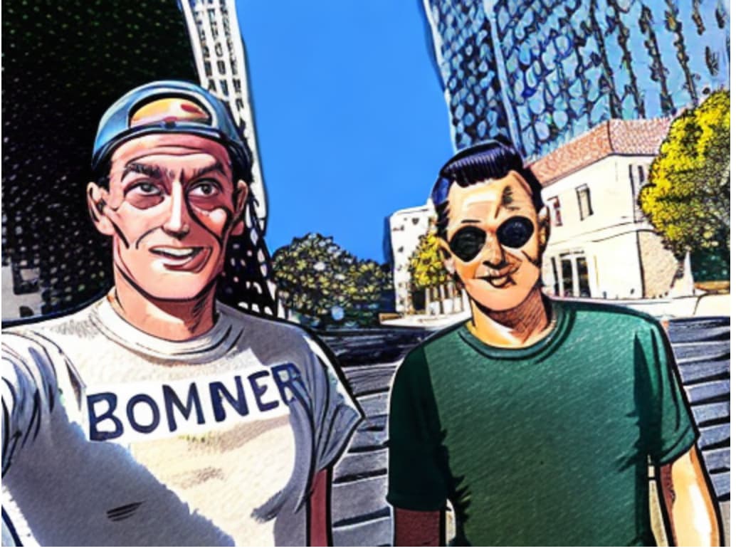
Below are some before/after images when combining all the 3 techniques together.
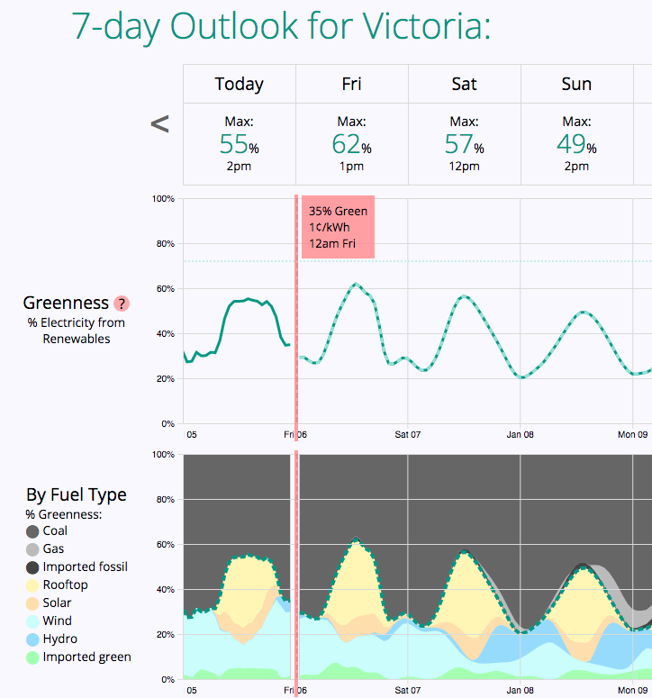
Sharing my fastai hobby project… greenforecast.au
May be particularly relevant to any Aussies out there?
Currently, the “greenness” of our electricity varies wildly throughout the day/week. I’m using fastai (and playing with miniai!!) to predict the next 7 days of “greenness” (and electricity price) in the hope that folks might reduce their carbon footprint, for example by:
choosing a ‘green’ time of day to charge an EV
‘overdrive’ heating/cooling during times of high greenness, reducing usage later
dream: a large scale user could take greenness into account when scheduling
dream: the nightly weather report includes a green forecast!
See the Q&A section of the site for the definition of “Greenness” and how it’s calculated
The ML is currently basic, I’m hoping to improve! So far most of the fun was building the custom dataset, fetching live data (input features) and hosting inference on AWS Lambda.
This is tabular* data, not images… apparently according to this excellent blog / list-of-papers, tabular datasets are where deep learning struggles the most against “traditional” techniques. Indeed my current best-performer is an ensemble of the fastai tabular learner (not much more than a 3 layer MLP!) and XGBoost. I’m lucky enough to have about ~1million datapoints, which apparently is where neural nets start to outperform the “old guard”.
*well technically I believe it’s “multivariate time series forecasting”
The site is here: http://greenforecast.au
Scroll down for “how I built this” Q&A and links to github.
Any feedback on either idea or execution is greatly appreciated!
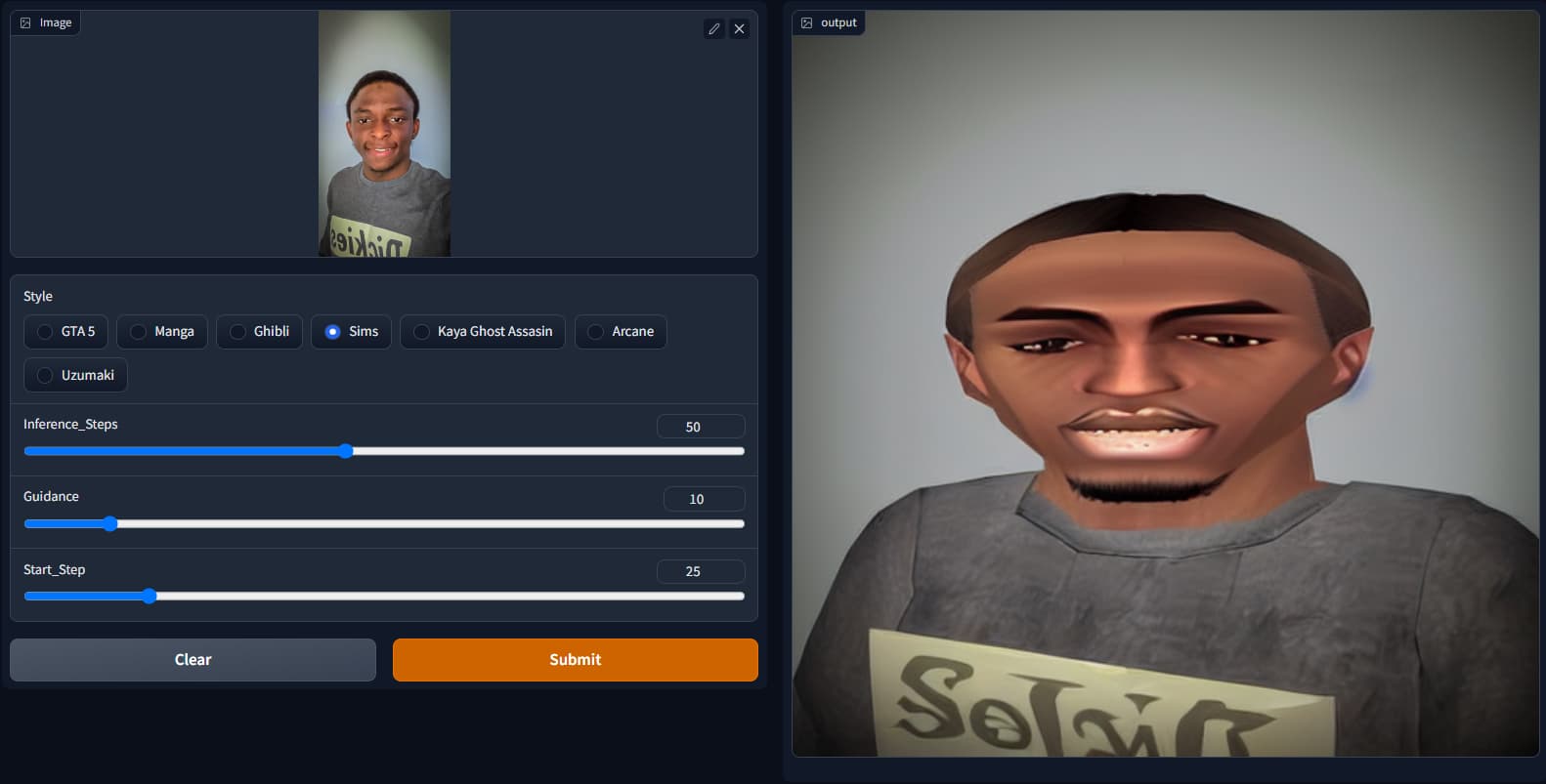
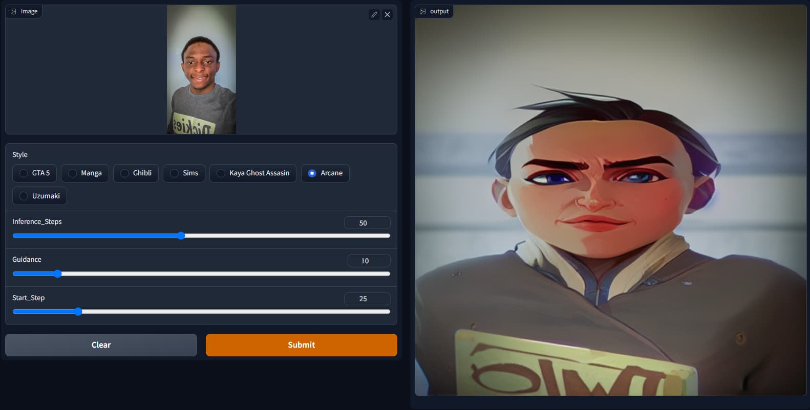
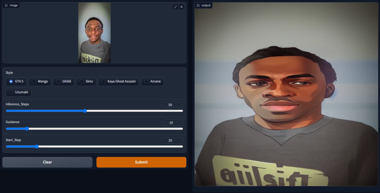
I’ve been playing with the SD notebook and I pieced together this img2img inpainting. There are 7 predefined styles you can choose from (got those from the sd-concepts-library). HuggingFace space for the app (It’s painfully slow though cause it’s running on a CPU instance)
@my0004, It looks a great foundation to build some good forecasting models, and a worthwhile topic to study. It would be interesting to see if the recent surge in energy prices can be seen to change behaviours and whether that could also be used as an input to the forecast, though I guess there will be a long lag
Since, this course is teaching stuff from the foundation, I started revisiting PyTorch and thought how cool it would be to write a book. Personally, writing things about a topic helps me solidify my own learning and forces me to really learn the topic. I have started writing a book about everything PyTorch, starting with the basics of PyTorch - The PyTorch Book (aayushmnit.com). Current chapters are equivalent of reading pytorch tutorials but with isolated examples per chapter explaining one single concept at a time.
In 2023, I will add a lot more chapters starting with NLP and semantic search. Hopefully people will find it useful.
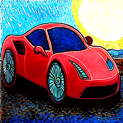
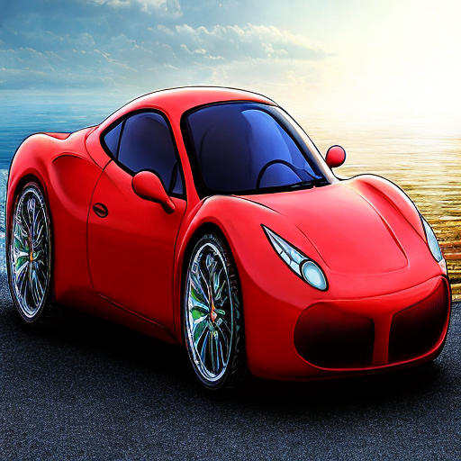
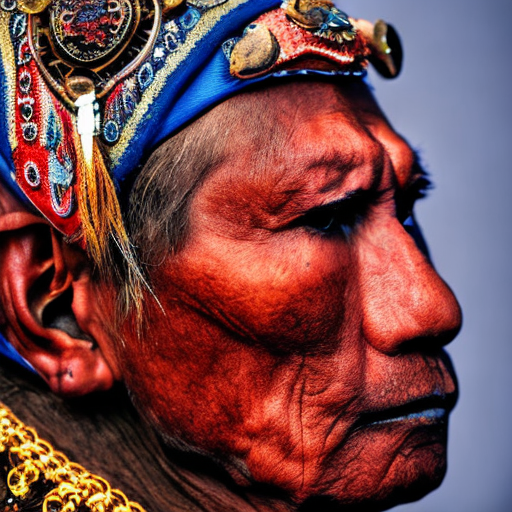
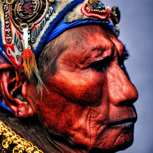
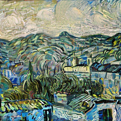
I’ve been continuing experimenting with generating images using style transfer with the loss additionally guided based on feature loss and style loss. I think these are quite an interesting result (with SD 2.1)
using a prompt of the description of van Gogh’s the starry night (which depicts a view of Saint-Rémy-de-Provence)
using the latents of an old photo of Saint-Rémy-de-Provence with added noise as the starting point.
included guidance to steer the style of the generated image to that of the starry night painting with VGG feature based gram matrix style loss within the loss for the generated image.
also included guidance to steer to attempt to help steer the latents to have similar features as the Saint-Rémy-de-Provence photo image used as a starting point with VGG feature loss as a small part of the loss.
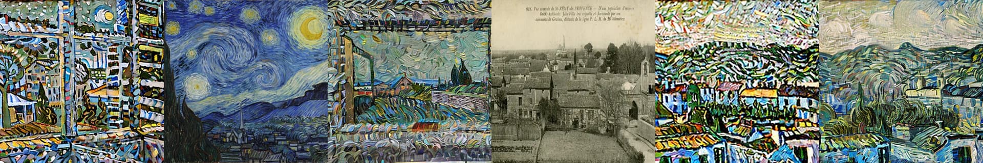
Within this its also scaling the loss for each of relevant VGG layers (before the max pooling layers) similar to those used in the super resolution loss function from the v3 course.
Showing a comparison from Left to right: (1) generated image only based on the prompt, (2) image used for style loss, (3) generated image from the prompt and feature style loss, (4) image for noisy starting latents, (5) generated image based on the prompt starting with the noisy image latents, (6) generated image based on the prompt starting with the noisy image latents using the feature loss and feature gram matrix style loss.
I’m going to continue tweaking this and put a blog post together with a notebook once I’ve tidied it up, if it is of interest.
It turns out not to be that a “piece of cake” to make this, but the blog is coming soon!
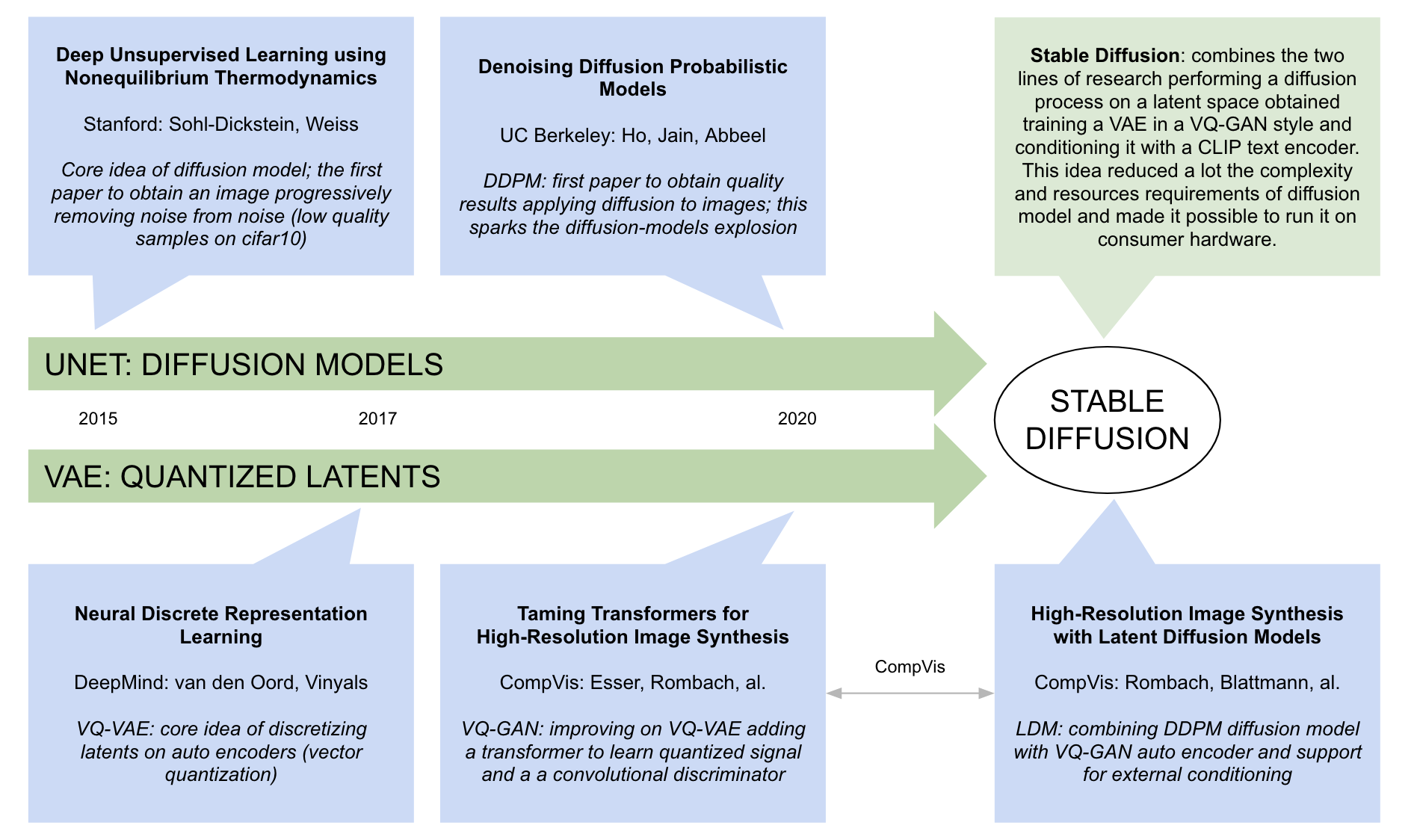
In the meantime I want to share my understanding of where Stable Diffusion comes from: did I forgot something?
Now depending on how detailed you want to get, you may also want to add the VAE, U-net, and CLIP papers too. And the CLIP text encoder is a transformer so you could add that too. Too many papers!
Yep I know… Just for joke I wanted to add backprop and alexnet
BTW: probably adding original DALL-E paper would be interesting, AFAIR they come out with the idea of learning with a transformer the tokens created by VQ-VAE.
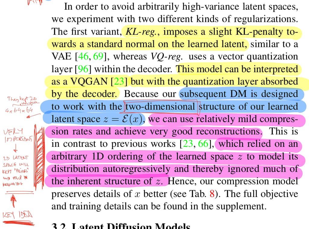
Eventually It seems they’ve chosen KL regularization (ie: stable_diffusion_deep_dive notebook uses AutoencoderKL).
Anyway, I would kept the reference to VQ-GAN paper at least for “historical reason” and because I think it’s interesting to track that CompVis group came out with a very popular image generation model almost a year before LDM.
BTW: Another interesting thing they hilighted here is the choice of a 2d latent space (4x64x64) instead of flattening to 1D sequence of tokens (like DALL-E and VQ-GAN) to let the diffusion model operate on a sort of latent pseudo image.