Thank you for your response, this also answers my second question. Now i understand.
The only part that i don’t exactly get it now is this part of this class:
class Lin():
    def __init__(self, w, b): self.w,self.b = w,b

    def __call__(self, inp):
        self.inp = inp
        self.out = inp@self.w + self.b
        return self.out

    def backward(self):
        self.inp.g = self.out.g @ self.w.t()
        # Creating a giant outer product, just to sum it, is inefficient!
        self.w.g = (self.inp.unsqueeze(-1) * self.out.g.unsqueeze(1)).sum(0)
        self.b.g = self.out.g.sum(0)
Here, we say: self.inp.g = self.out.g @ …
As i know ‘=’ this operator assigns right hand side to left hand side.
But here we never assign anything on self.out.g (since we never put it on left hand side).
It is like we didn’t define self.out.g . How this code get away with this?
So i tried to implement this on my simple code like this:
Lin/ReLU or any layer during forward propagation will never use backward()… only when MSE is invoked there is a need to calculate gradient (g).
So in Model class, MSE will be the loss that will instantiate ‘g’ and will store the gradient values from there on. Next, ReLU layer will be invoked where this outoput of MSE (along with g) will be passed. Same for Lin layer - and hence backward function through the tensor will have access to g.
Right before the broadcasting section at the 51:00 mark, how is it just 178 times faster? Shouldn’t it be 831/1.4 = 593 times faster? Where did the 890.1/5 come from? I don’t see anything mentioned in the errata either.
Hi everyone, I have written a blog to help people understand the intuition behind BLAS processor libraries that break down matrix multiplications. Jeremy mentioned this as a reason for the pytorch matmul() function’s superior execution speed. The blog will describe a simple way to break down matrix multiplications into several parts. Hope this helps someone.
Hi everyone. I wrote up my own notes on this lesson. This took several days to write because I got bogged in the backpropagation section. It took a while to convince myself that I could derive the expressions for the derivatives. I wrote with quite a bit of detail here with many links to things that made it all ‘click’ for me. I hope that my write-up helps it to click for someone else too! James
I am hoping somebody can help me because I am banging by head against a brick wall
I am using the RetinaNet notebook for object detection, after running different experiments my results were getting worse and no where near what I got the first time round so I decided to do a check.
I looked at the model where I got good reults, an mAP of 0.36
So I took tha same model, same notebook, same data, changed NOTHING and my results are terrible mAP 0.15. Has anyone come across this before ? I haven’t changed a thing but I know that something must be different and I can’t seem to find out what it is!.
Thanks
Hi, as I was trying to reproduce the notebook of the lesson I stumbled upon the backward implementation.
I finally got to understand it and I figured I would share how I got there. It is a pretty simple and step by step walk through but it might be helpful for some one.
After many months, I have finally decided to go through part 2 of the course for the second time, this time slowing down, and trying to dive deep and replicate all the code. I have gone through the posts in this topic and since it seems that the thing has been unanswered, I can through my 2p on the reason why in pytorch the weight of the linear module are stored transposed.
I can think of two possible explanations, somewhat related. We know that a linear transformation from a space of dimension n_{in} to a space of dimension n_{out} can be described both as A \mathbf x or \mathbf v B where A has shape (n_out, n_in) while B has shape (n_in, n_out) and \mathbf x is a column vector, while \mathbf v is a row vector. The first form is more common in geometry and it is what I would think of as the transformation matrix of the linear map.
There is also the age old question of how to write composed functions.
Say that we have two linear functions f and g that we that we want to apply to a pandas Series. We can write it both as g(f(series)) and series.apply(f).apply(g). If we consider the weights matrix like pytorch, the resulting linear transformation is the linear transformation has weight W_g W_f, which is more natural in the first case (as we multiply the weights in the same order as we write the functions), but the second way looks weird. On the other hand, if we store the weights as we did in the lecture, the second way of composing is more natural, as the resulting weight matrix would be W_f W_g. In maths there is no right way of doing it, but mathematicians tend to be very opinionated about the subject depending on the field they are working on. Personally I feel that with Deep Learning, one way is more convenient at inference time (the pytorch way), while the other is more convenient at training time (the lesson 8 way).
Of course there might be hidden implementation reasons, and I might be completely wrong. Apologies for the wall of text.
Hello! I’m sorry, I don’t quite understand your explanation. Would you mind clarifying a bit? Like @hwqwn, I am also confused about how the backward() function is able to access self.out.g. Can you please point out the specific way that the self.input.g from the next layer somehow becomes accessible as self.output.g in the previous layer? I have looked at the code for hours but still can’t see why this should be possible. Thank you!
at the forward pass, you render each layers output to the next layer as input. For example, if you get output from first linear, that would be input of ReLU at the same time.
In the same way, second linear layer’s output will be rendered to input of Mse
at the backward process, when you call loss.backward(), that method would assign .g attribute to the mse’s input which was at the same time linear 2’s output.
I just made dummy example, which shows what I wanted to explain. hope this helps someone
class first():
    def __init__(self, a, b):
        self.a, self.b = a, b
    def __call__(self):
        self.out = self.a + self.b
        return(self.out)

class second():
    def __init__(self, inp):
        self.inp = inp
    def __call__(self):
        self.inp.g = self.inp * .5
        return(self.inp)

f = first(torch.tensor(10), torch.tensor(3))
f(), f.out
>>> (tensor(13), tensor(13))
f.out.g

>>> AttributeError Traceback (most recent call last)

[<ipython-input-26-e38ce6ee9d5d>](https://localhost:8080/#) in <module>() ----> 1 f.out.g

AttributeError: 'Tensor' object has no attribute 'g'
You don’t have g attribute yet, but
s = second( f() )
s()
>>> tensor(13)
After you give a result of first class, and then call the second instance, which will assign g attribute, and now you can get
I just worked my way through class8. It is really a fascinating class! However I have some questions about the resnet paper and also Jeremy’s class (I think there might be a mistake too) @jeremy Question about Resnet paper:
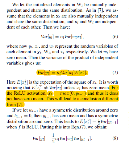
in section 2.2 Forward Propagation Case, in order to be able to reach conclusion[7] Var[y_{l}] = n_{l}Var[w_{l}]E[x_{l}^{2}], x_{l} and w_{l} has to be two independent random variables, which is not the case when x_{l} is ReLU output. The paper actually pointed out that for ReLu activation, it does not have zero mean and this will lead to a different conclusion; However I do not understand why they still go ahead and recommended \sqrt{\frac{2}{n_{l}}} as the standard deviation for initialization? in practice, with the 2-hidden layer example we used in this class, I found that the relationship between Var[y_{l}] and w_{l} and x_{l} is more like this:Var[y_{l}] = \frac{1}{2} n_{l}Var[w_{l}]E[x_{l}^{2}] (when [y_{l}] is lin(relu(lin(x,w1,x1) ),w1,x2)) in the 2-hidden FC layer example, w_{l} is w2, and x_{l} is (relu(lin(x,w1,x1))
so this lead to my questions about this particular part in Jeremy’s class where he used below example to demo that by using kaiming init you can get std to close to 1 (see the code from notebook below) : here t1 is a ReLU activation (defined as in t1 = relu(lin(x_valid, w1, b1))), I think t1 is the x_{l} in the resnet paper. and the variance of t1 is not suppose to be same as y_{l-1}, it should be slightly higher than 0.5var(y_{l-1}) , I think we should check lin(relu(lin())) instead
def relu(x):
    return x.clamp_min(0.) - 0.5


for i in range(10):
    # kaiming init / he init for relu
    w1 = torch.randn(m,nh)*math.sqrt(2./m )
    t1 = relu(lin(x_valid, w1, b1))
    print(t1.mean(), t1.std(), '| ')
To continue my last post, because we were tracking the variance and mean of the wrong output the experiment we did in class 8 with **def relu(x): return x.clamp_min(0.) - 0.5** would actually lead to a very different conclusion: even though the ReLU activation has mean around 0.5, the mean of y_{l} (e.g. t could be lin(x1,w1,b1) or lin(relu(lin(...)...) or lin(relu(lin(...)...)...) and so on) is actually around 0 so we did not actually need to do anything to adjust it; plus by substract 0.5 from the ReLU activation, it breaks the math between E(x^{2}) and variance of previous linear’s output y_{l-1} -i.e. E(x^{2}) \neq \frac{1}{2}var[y_{l-1}] if you check the variance of y_{l} you will find it will not able to remain same even with kaiming initialization (when you substract 0.5 from ReLU activation)
Here is the testing I did -
this is the benchmark, you can see y1.var and y2.var is quiet close
def relu(x): return x.clamp_min(0.)
nh1 = 50
nh2 = 25
for i in range(10):
    # kaiming init / he init for relu
    w1 = torch.randn(m,nh1)*math.sqrt(2./m )
    b2 = torch.zeros(nh1)
    w2 = torch.randn(nh1,nh2)*math.sqrt(2./nh1 )
    b2 = torch.zeros(nh2)
    y1 = lin(x_valid, w1, b1)
    x2 = relu(y1)
    y2 = lin(x2, w2,b2)
    print(y1.std(), y2.std(), '| ')

tensor(1.3692) tensor(1.4562) |
tensor(1.3973) tensor(1.2707) |
tensor(1.3976) tensor(1.5857) |
tensor(1.3961) tensor(1.3642) |
tensor(1.5039) tensor(1.6659) |
tensor(1.3697) tensor(1.5277) |
tensor(1.3700) tensor(1.2482) |
tensor(1.4665) tensor(1.2678) |
tensor(1.4137) tensor(1.5692) |
tensor(1.4276) tensor(1.4433) |

This is the testing when we substract `0.5` from ReLu activation, you can see `y2.var` is not so close to `y1.var`


def relu(x): return x.clamp_min(0.) - 0.5
nh1 = 50
nh2 = 25
for i in range(10):
    # kaiming init / he init for relu
    w1 = torch.randn(m,nh1)*math.sqrt(2./m )
    b2 = torch.zeros(nh1)
    w2 = torch.randn(nh1,nh2)*math.sqrt(2./nh1 )
    b2 = torch.zeros(nh2)
    y1 = lin(x_valid, w1, b1)
    x2 = relu(y1)
    y2 = lin(x2, w2,b2)
    print(y1.std(), y2.std(), '| ')
tensor(1.4030) tensor(1.1121) |
tensor(1.3632) tensor(1.0190) |
tensor(1.4385) tensor(1.2674) |
tensor(1.4606) tensor(1.1940) |
tensor(1.3023) tensor(0.9659) |
tensor(1.4748) tensor(1.2869) |
tensor(1.3788) tensor(1.1413) |
tensor(1.3320) tensor(1.1093) |
tensor(1.3915) tensor(1.0241) |
tensor(1.3817) tensor(1.0187) |