Thanks for your answer, Jeremy!
May I ask you for a brief comment about the second part (the one where you were talking about the loss surface topology and their stationary points).
Thanks! 
Thanks for your answer, Jeremy!
May I ask you for a brief comment about the second part (the one where you were talking about the loss surface topology and their stationary points).
Thanks!
Yes I think that’s about right. I’m not sure my comment about this or this overall part of the discussion was particularly helpful though.
I bet it was. Pushed me to reasoning about such matter, anyhow. Thanks!
Trouble install part2 on local Ubuntu 19.04. Anyone have instruction?
Only just a note if someone tried
conda install fire -c conda-forge
in google cloud and it didn’t work and display
InvalidArchiveError(‘Error with archive /opt/anaconda3/pkgs/certifi-2019.6.16-py37_0.tar.bz2. You probably need to delete and re-download or re-create this file. Message from libarchive was:\n\nCould not unlink (errno=13, retcode=-25, archive_p=93938759495040)’)
InvalidArchiveError(‘Error with archive /opt/anaconda3/pkgs/conda-4.7.5-py37_0.tar.bz2. You probably need to delete and re-download or re-create this file. Message from libarchive was:\n\nCould not unlink (errno=13, retcode=-25, archive_p=93938760719088)’)
in the bottom. just change it to
pip install fire
and it will work finely when trying 00_exports.ipynb for exporting .py files.
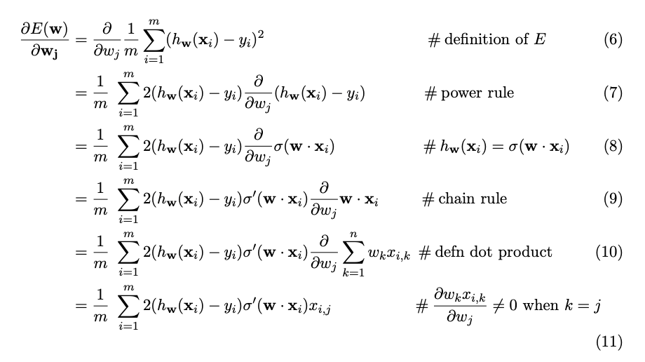
Here is a great explanation of gradient of MSE in matrix form which I found here.
We take partial derivative with respect to weights Wj and here sigma is the activation function. Since we are using RELU, the derivative is 1 when positive and zero otherwise in eq.(11).
Since, summation is from 1 to m, which is positive numbers, the term ![image|97x35]
(upload://oJG7gEDfHJv2zpL9Sw8ozr2PtHS.png) becomes 1 as it is RELU activation function.
So finally, we are left with 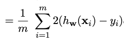 which equates to
 2. * (inp.squeeze() - targ).unsqueeze(-1) / inp.shape[0] in code.
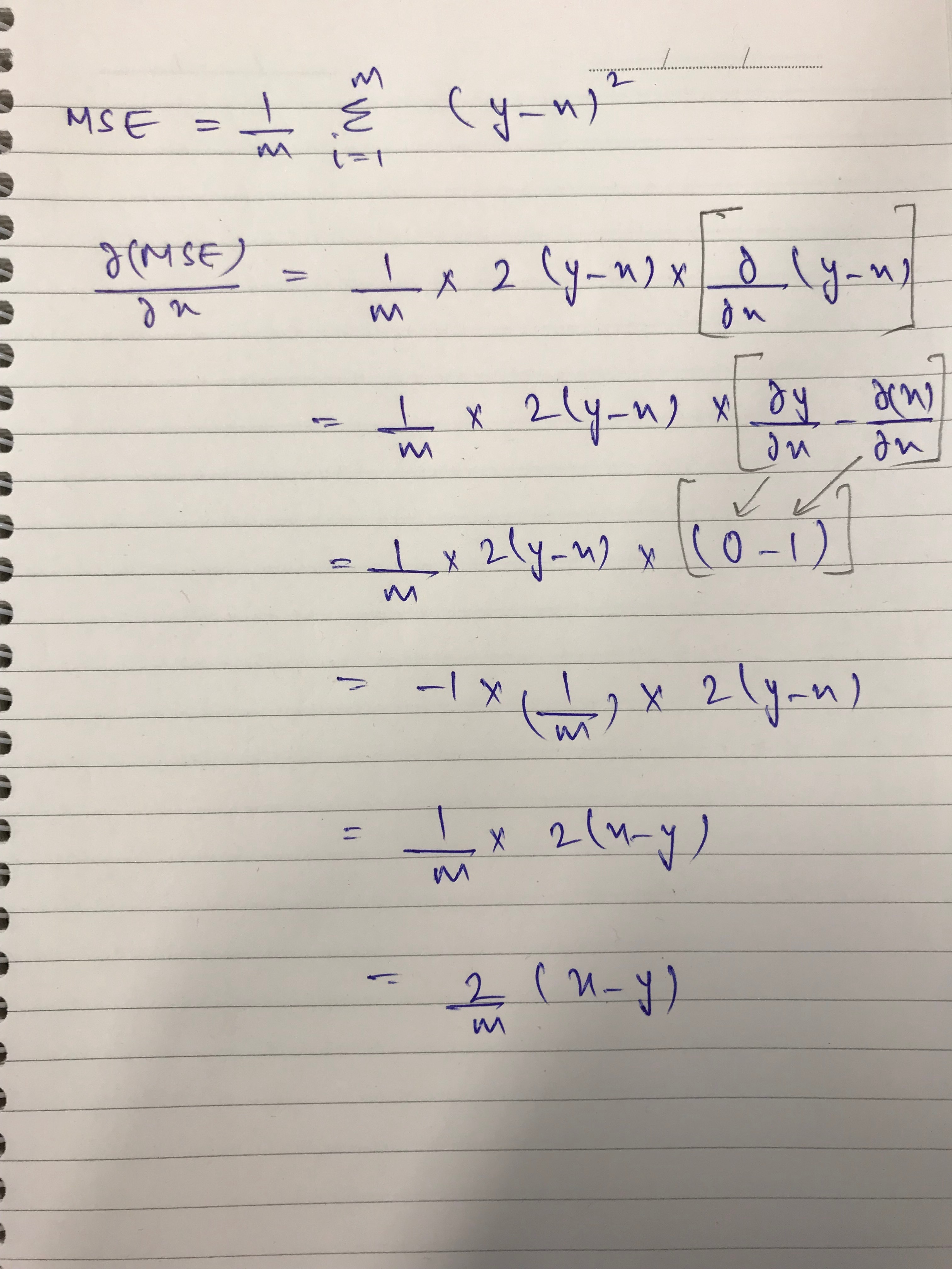
CORRECTION
Correct derivation for gradient of MSE:
Thanks for posting this clear deivation.
One comment: your reasoning that the relu can be set to one “Since, summation is from 1 to m, which is positive numbers” is confusing, as m indexes the example number, and is not the argument of the relu. Also, how did factor of x_ij disappear?
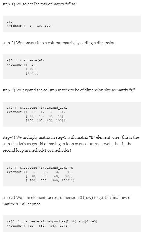
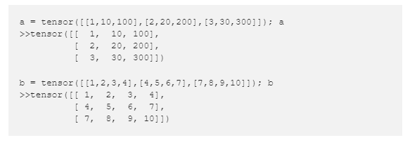
Hi all, I’ve written an article explaining matrix multiplication in detail here. It explains the broadcasting line of code used in method-3 step by step. Always happy to get feedback from the community!
Thanks for the great question @jcatanza. In order to find an answer for your question, I dug deep into the matrix calculus paper provided by Jeremy here and found a mistake in my previous post.
Please find the hand derived formula for the gradient of MSE as below:
Note: This is a partial derivative of MSE with respect to output of prev class (x). Since, y represents target, which is a scalar, its derivative becomes 0.
Hope this helps!
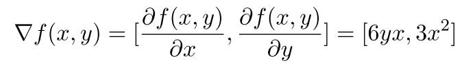
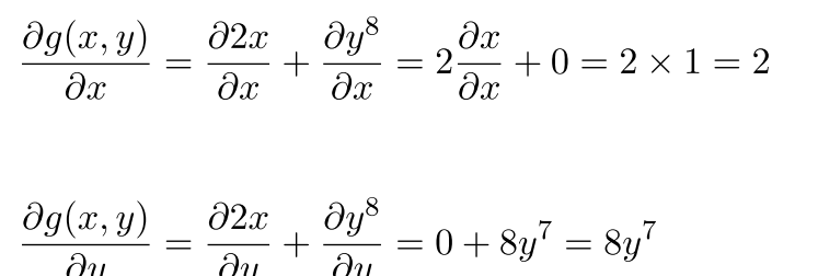
I am reading the Matrix calculus paper . In section 3 calculating partial derivative of a function is shown like below.
While taking partial derivative of the function f(x,y) which is 3x2, we have considered y as a constant and the partial derivative wrt x is 6yx. In section 4 while calculating partial derivative for another function g(x,y) = 2x + y8 with respect to x, the partial derivative of y8 wrt x becomes 0 like shown below.
Should it not be 2y8. Am I missing something here ?
In your first example, I am assuming the original example was (3x^2)(y). With respect to x, this yields 6xy since y is a constant like you said. With respect to y, this is just 3x^2.
In the one you are stuck with, our function is 2x + y^8. Since we are adding, we lose the variable if we treat it as a constant when we take the derivative. So, with respect to x, this becomes 2. With respect to y, we drop the 2x (because it is a constant) and only look at the y^8, which has a derivative of 8y^7. The difference here is that we are adding in this example versus multiplying in the first.
Hope this helps!
Thanks I missed the addition part. Got it now.
Thanks for sharing! ![]() One thing to mention - you’ve copied an image from a book that’s watermarked “not for redistribution”. You should probably replace that with a version you create yourself, or from some other source that doesn’t have that restriction.
One thing to mention - you’ve copied an image from a book that’s watermarked “not for redistribution”. You should probably replace that with a version you create yourself, or from some other source that doesn’t have that restriction.
Thanks so much @jeremy for the feedback! 
It just made my day and I feel more motivated about writing blogs.
I have updated the article and used Excel to explain all the three matrix multiplication methods including Broadcasting. Google sheet version for the same can be found here.
I like the Excel walkthru! Oh BTW Rachel didn’t create the song. I’m not sure where it originally came from.
Thanks @jeremy for putting effort and preparing the materials. I found it very useful. I think there are two very good resources that can accompany the second half the lecture about preprocessing and initialization.
At time 01:45:30 @jeremy said that subtracting 0,5 from relu helped to stabilize the variance. Is that correct? Because adding a constant to a random variable doesn’t change its variance.
Just a little remark: At 01:55:00 in the backpropagation:
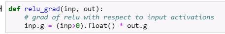
The comment says that its the gradient of relu with respect to input activations.
Shouldn’t it be the gradient of the loss with respect to the activation? Since we’ve multiplied by out.g (that’s the chain rule to compute the gradient of the loss)
I don’t think he was talking about the RV variance, but the RV mean. I’ll double check though.
Hi!
Could someone explain why the gradient of a matrix is its transpose?
I read the paper about matrix calculus mentioned in the video but wasn’t able to find the answer.
Edit: More specifically, I am trying to understand this piece of code:
def lin_grad(inp, out, w, b):
# grad of matmul with respect to input
inp.g = out.g @ w.t()  #???
If my understanding is correct, at the final layer of the network, inp.g is the gradient of the layer’s output with regards to the layer’s input, i.e. ReLU(w1.x + b1). In this case, the output is a vector of dimensions (N, 1) with N = number of training examples.
The input is a matrix of dimensions (N, nh) (with nh = 50).
So is this a case of computing the derivative of a vector w.r.t. a matrix? Which is not a case covered in any material I managed to find online (they do not go beyond matrix by scalar or scalar by matrix).
Intuitively, I would imagine the resulting gradient to be a rank-3 tensor because we’re computing the partial derivative of each element of the vector w.r.t. each element of the matrix.
I don’t quite get where the formula in the code comes from. If anyone could provide some insight, I would be very grateful!