Lesson 6 In-Class Discussion ✅

The log error log(y) - log(yhat), this is the same as log(y / yhat).

We use the trick of adding 0: y / yhat is the same as y / yhat + (1 - yhat/yhat) which is the same as 1 + (y - yhat) / yhat where the second term is the percent error (PE).

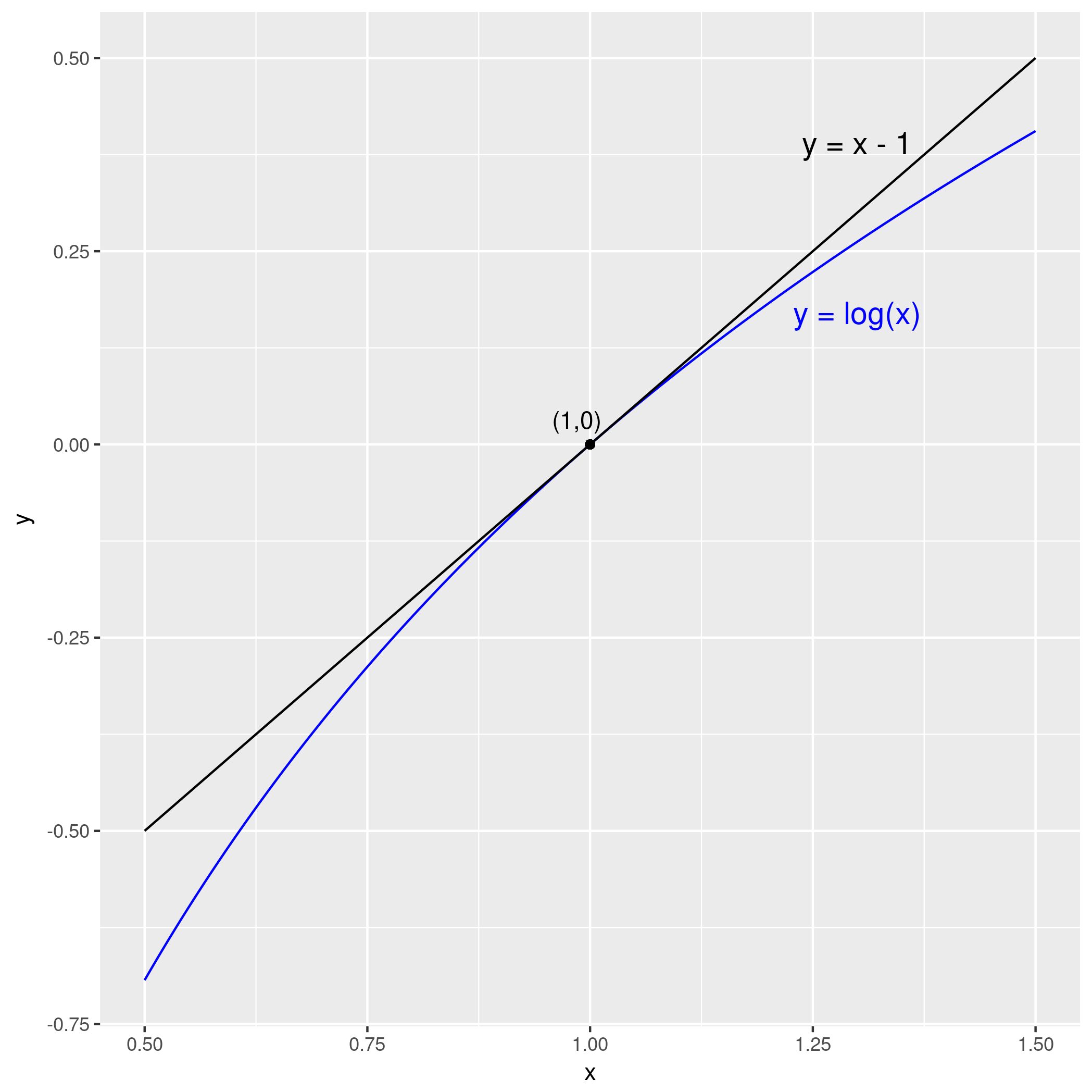
So log(y) - log(yhat) is the same as log(1 + PE), which is approximately PE when PE is small (as you can verify with a plot).

So log(y) - log(yhat) is approximately the same as (y - yhat) / yhat when either result is much smaller than 1.

So when your predictions are pretty good you get log error is almost the same as percent error, as you can verify experimentally, and you should get similar final model accuracy.

13 Likes

Thank you! That’s fabulous!

You can treat categorical variables in the same way you treat “words” when training a language model (words are effectively categorical variables).
So you can for example keep all the values with a minimal frequency of 3 and substitute with “RARE” the values that appears less than 3 times…

Jeremy cited “Vtreat” package for R in the previous course: in the paper you can find some exmaple of how to deal with “RARE” values.
https://arxiv.org/abs/1611.09477

I’m running the pets-more notebook and when going through the Grad-CAM section it can’t find the image bulldog-maine.jpg. I see that we’re looking for it in fn = path/'../other/bulldog_maine.jpg' but there isn’t an other folder within oxford-iiit-pet. Any ideas where I can find the image?

Thank you! I never thought of it that way and it makes a lot of sense. The paper was great!

Wow this is mind bending. This could be a great way for generalization. Reminds of adversarial training.

2 Likes

I think the author is misleading the readers. What you see is part of a pachyderm (read elephant) with a cat tattoo or cat etching. I am going to try and make the background grass and feed it to a classifier and then see what it comes up with.

1 Like

The second image is pretty undeniable. And in your agrument, it should have given a higher raw score to cat as well as elephant to make it not that confident.

The point is that earlier layers are easily fooled as they have small kernals. And once they are fooled that info is only propagated forwards.

Here is the proof.
I fed the cat image with a green background (I also had to do a gaussian blur since my manual lasso selection of the edge was quite pointy at ears) to TensorFlow.js demo and got

label prob
Egyptian cat 0.38
tabby, tabby cat 0.36
tiger cat 0.07

Conclusion is that the cat was recognized inspite of it’s pachyderm texture !!

The Tensorflow.js demo was at

3 Likes

Interesting! I’m sure the author might be interested in your work. I wonder if there is no other category in the model that matches the green, it may not disprove their hypothesis, but it does perhaps show that absent of texture, shape can still match successfully.
That said, I agree that their proof that the texture drives the classification is not air tight. However, I appreciated their approach to augmenting the images to prevent dependence on texture.

1 Like

I think your analysis in the comments of the post is incorrect. The fooling images work by making the first few layers with small receptive field size show very high activations towards a particular class. Then this is the information that gets propagated forwards as the input is lost. The activations are so high(across the whole h and w), in this case for elephant skin, that the feature detectors show strong evidence for that class. Green may be not raise very high activations towards any particular class allowing the shape to have a relatively high activation.

The green background is just my laziness. I could have had some indoor couch as the bacground. My disagreement with the authors is that they are applying the texture on the background as well. What do we want the classifier to do in such cases?. Specifically if I manage to find an elephant with a cat that the elephant has fallen in love with tattooed on its rump. I take a close photo of that cat. What do I get? Pachyderm background as well as pachyderm texture on the cat. That is exactly the image we have to begin with. Now what should the model predict this image as? You would say elephant ! That is exactly what it does !!

Most cats in imagenet cats are furry sitting on non-furry backgrounds. My green background cat is not furry at all. It has the pachyderm texture all over it. But the model still called it cat based on the shape it saw (giving lower weight to its pachyderm texture). This in my mind calls for the authors to restate their hypothesis.

1 Like

Lols, yes I agree. Pachyderm with cat tattoos! It is a good point.

You should just pick any image you like. I searched google images to find one for the lesson.

1 Like

Thank you. That’s helpful. Is this averaging done depending on the application. I am just thinking that averaging will lead to loss of overall information (for example, we might end up averaging different pixel intensities which might be okay for games but not ok for medical images?) - Probably there’s some reasoning as to how average pooling preserves accuracy that I am not getting?

Does the model using the Rossman dataset use all of the columns in the train_df pickle file? Or only the subset defined in the cont_vars and cat_vars? I ask this because:

len(train_df.columns)
93
len(cat_vars + cont_vars)
38

Hi,

noob python question. The TabularModel class takes arguments emb_szs and n_cont without any default set. In the Rossman notebook, the learner is created without setting these. How does this work?

Tabular Model init:

class TabularModel(nn.Module):
"Basic model for tabular data."
def __init__(self, emb_szs:ListSizes, n_cont:int, out_sz:int, layers:Collection[int], ps:Collection[float]=None,
             emb_drop:float=0., y_range:OptRange=None, use_bn:bool=True, bn_final:bool=False):
    super().__init__()
    ps = ifnone(ps, [0]*len(layers))
    ps = listify(ps, layers)
    self.embeds = nn.ModuleList([embedding(ni, nf) for ni,nf in emb_szs])
    self.emb_drop = nn.Dropout(emb_drop)
    self.bn_cont = nn.BatchNorm1d(n_cont)
    n_emb = sum(e.embedding_dim for e in self.embeds)
    self.n_emb,self.n_cont,self.y_range = n_emb,n_cont,y_range
    sizes = self.get_sizes(layers, out_sz)
    actns = [nn.ReLU(inplace=True)] * (len(sizes)-2) + [None]
    layers = []
    for i,(n_in,n_out,dp,act) in enumerate(zip(sizes[:-1],sizes[1:],[0.]+ps,actns)):
        layers += bn_drop_lin(n_in, n_out, bn=use_bn and i!=0, p=dp, actn=act)
    if bn_final: layers.append(nn.BatchNorm1d(sizes[-1]))
    self.layers = nn.Sequential(*layers)

Defining learner in Rossman notebook:

learn = tabular_learner(data, layers=[1000,500], ps=[0.001,0.01], emb_drop=0.04, 
                    y_range=y_range, metrics=exp_rmspe)

How can we check what value will be better for our pct_start? Is there any way to find it or just some hit and trials. Also when we should put bn_final=True?

Dig into the code a little deeper and you’ll see how tabular_learner constructs the TabularModel

def tabular_learner(data:DataBunch, layers:Collection[int], emb_szs:Dict[str,int]=None, metrics=None,
        ps:Collection[float]=None, emb_drop:float=0., y_range:OptRange=None, use_bn:bool=True, **kwargs):
    "Get a `Learner` using `data`, with `metrics`, including a `TabularModel` created using the remaining params."
    emb_szs = data.get_emb_szs(ifnone(emb_szs, {}))
    model = TabularModel(emb_szs, len(data.cont_names), out_sz=data.c, layers=layers, ps=ps, emb_drop=emb_drop,
                         y_range=y_range, use_bn=use_bn)
    return Learner(data, model, metrics=metrics, **kwargs)

How do we deal with binary variables which do not have NA? Do we consider them as categorical variable of cardinality 2 and stick it into an embedding matrix or do we consider them as a real value as part of continuous variables?