Fast.ai v3 2019课程中文版笔记

Daniel · March 11, 2019, 11:27am

MNIST SGD

所需library

%matplotlib inline
from fastai.basics import *

点击下载数据集

Get the ‘pickled’ MNIST dataset from http://deeplearning.net/data/mnist/mnist.pkl.gz. We’re going to treat it as a standard flat dataset with fully connected layers, rather than using a CNN.

查看数据文件夹

path = Config().data_path()/'mnist'

path.ls()

[PosixPath('/home/ubuntu/.fastai/data/mnist/mnist.pkl.gz')]

解压pkl数据包

with gzip.open(path/'mnist.pkl.gz', 'rb') as f:
    ((x_train, y_train), (x_valid, y_valid), _) = pickle.load(f, encoding='latin-1')

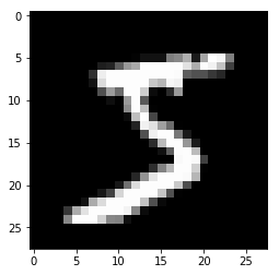
展示图片和训练数据shape

plt.imshow(x_train[0].reshape((28,28)), cmap="gray")
x_train.shape

(50000, 784)

output_12_1

将训练和验证数据转化为torch.tensor

x_train,y_train,x_valid,y_valid = map(torch.tensor, (x_train,y_train,x_valid,y_valid))
n,c = x_train.shape
x_train.shape, y_train.min(), y_train.max()

(torch.Size([50000, 784]), tensor(0), tensor(9))

In lesson2-sgd we did these things ourselves:

x = torch.ones(n,2) 
def mse(y_hat, y): return ((y_hat-y)**2).mean()
y_hat = x@a

Now instead we’ll use PyTorch’s functions to do it for us, and also to handle mini-batches (which we didn’t do last time, since our dataset was so small).

将X与Y(torch.tensor)整合成TensorDataset

bs=64
train_ds = TensorDataset(x_train, y_train)
valid_ds = TensorDataset(x_valid, y_valid)

将训练和验证集的TensorDataset 整合成DataBunch

data = DataBunch.create(train_ds, valid_ds, bs=bs)

从训练集DataBunch中一个一个提取数据点

x,y = next(iter(data.train_dl))
x.shape,y.shape

(torch.Size([64, 784]), torch.Size([64]))

创建模型的正向传递部分

class Mnist_Logistic(nn.Module):
    def __init__(self):
        super().__init__()
        self.lin = nn.Linear(784, 10, bias=True)

    def forward(self, xb): return self.lin(xb)

启用GPU机制

model = Mnist_Logistic().cuda()

查看模型

model

Mnist_Logistic(
  (lin): Linear(in_features=784, out_features=10, bias=True)
)

调用模型中的lin层

model.lin

Linear(in_features=784, out_features=10, bias=True)

模型输出值的shape

model(x).shape

torch.Size([64, 10])

调取模型每一层的参数，查看shape

[p.shape for p in model.parameters()]

[torch.Size([10, 784]), torch.Size([10])]

设置学习率

lr=2e-2

调用分类问题损失函数

loss_func = nn.CrossEntropyLoss()

一次正向反向传递计算函数详解

def update(x,y,lr):
    wd = 1e-5
    y_hat = model(x)
    # 设置 weight decay
    w2 = 0.
    # 计算 weight decay
    for p in model.parameters(): w2 += (p**2).sum()
    # 将 weight decay 添加到 常规损失值公式中
    loss = loss_func(y_hat, y) + w2*wd
    # 求导
    loss.backward()

    # 利用导数更新参数
    with torch.no_grad():
        for p in model.parameters():
            p.sub_(lr * p.grad)
            p.grad.zero_()
    # 输出损失值
    return loss.item()

对训练集中每一个数据点做一次正反向传递（即SGD），收集损失值

losses = [update(x,y,lr) for x,y in data.train_dl]

将损失值作图

plt.plot(losses);

output_43_0

构建一个2层模型，第一层含非线性激活函数ReLU

class Mnist_NN(nn.Module):
    def __init__(self):
        super().__init__()
        self.lin1 = nn.Linear(784, 50, bias=True)
        self.lin2 = nn.Linear(50, 10, bias=True)

    def forward(self, xb):
        x = self.lin1(xb)
        x = F.relu(x)
        return self.lin2(x)

开启GPU设置

model = Mnist_NN().cuda()

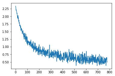
用SGD计算获取训练集的损失值，并作图

losses = [update(x,y,lr) for x,y in data.train_dl]

plt.plot(losses);

output_50_0

再次开启模型的GPU计算模式

model = Mnist_NN().cuda()

正反向传递中加入Adam优化算法和opt.step()取代手动参数更新公式

def update(x,y,lr):
    opt = optim.Adam(model.parameters(), lr)
    y_hat = model(x)
    loss = loss_func(y_hat, y)
    loss.backward()
    opt.step()
    opt.zero_grad()
    return loss.item()

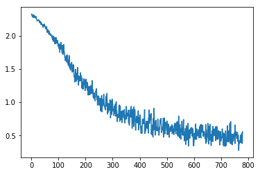
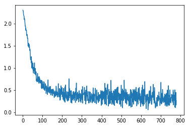
对训练集做SGD，收集损失值，并作图

losses = [update(x,y,1e-3) for x,y in data.train_dl]

plt.plot(losses);

output_57_0

采用fastai Learner方式进行建模

learn = Learner(data, Mnist_NN(), loss_func=loss_func, metrics=accuracy)

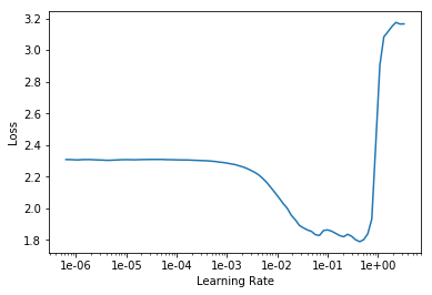
作图寻找学习率最优值

learn.lr_find()
learn.recorder.plot()

LR Finder is complete, type {learner_name}.recorder.plot() to see the graph.

output_61_2

挑选最优值学习率，进行训练

learn.fit_one_cycle(1, 1e-2)

Total time: 00:03

epoch	train_loss	valid_loss	accuracy
1	0.129131	0.125927	0.963500

画出学习率和momentum图

learn.recorder.plot_lr(show_moms=True)

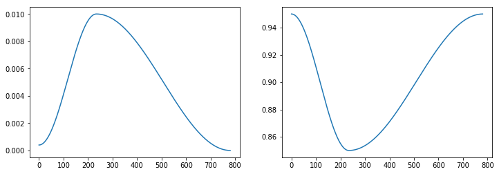
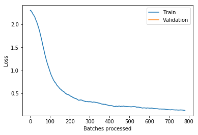
画出损失值（训练vs验证）图

learn.recorder.plot_losses()

output_67_0