Algoritmos de otimização do Gradient Descent (GD)
-
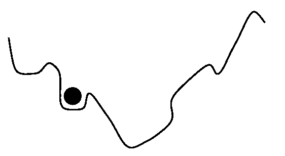
momentum : the force that keeps an object moving or keeps an event developing after it has started (momentum can be seen as a ball running down a slope) - Leia artigo “Stochastic Gradient Descent with momentum”.
- Adam (Adaptive Moment Estimation) + “Gentle Introduction to the Adam Optimization Algorithm for Deep Learning” : ADAM creates an adaptative learning rate
-
Regularization : avoid overfitting by regularization of the weights values (video from Andrew Ng)
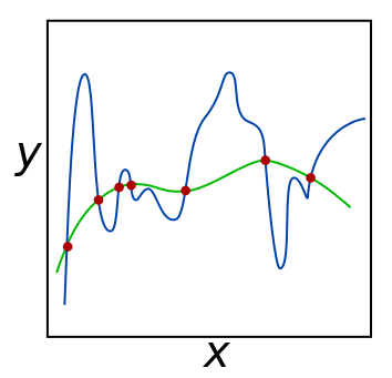
The green and blue functions both incur zero loss on the given data points. A learned model can be induced to prefer the green function, which may generalize better to more points drawn from the underlying unknown distribution, by adjusting {\displaystyle \lambda } \lambda , the weight of the regularization term. - L2 regularization (weigh decay)
- ADAMW : New AdamW optimizer now available