I’ve seen lots of scattered discussions on the Rossmann notebook, mostly debugging and learning the basics.
I wanted to open a thread to see what people have tried in terms of improving on the result.
The first obvious step is correcting the mistake Jeremy highlighted where they dropped all rows where sales =0
This isn’t 100% straightforward because leaving those rows in the dataframe means you start running into dividing by 0 errors in the evaluation function that’s written.
Another step, very much related to the first but something I haven’t seen other people talk about is doing before and after feature engineering counters on the event of a store being open or not. The EDA on this dataset shows this is important so making it easier to see should help the model. I also wonder why the authors chose so few of their features to use. Prior to creating lists of cat_vars and contin_vars there were 95 features. Then the lists reduce that down to 38. Why not keep these and try L2 regularization or other approaches to preventing over fitting.
Once the fix to the sales = 0 issue has been implemented, it seems like the next best step is to follow the ML1 approach of running a random forest as fast as possible and doing EDA via random forests feature importance and seeing if there is additional valued-added feature engineering to be done. Additionally, as noted in the videos, it seems like passing in the categorical embeddings to the Random Forest increases it’s performance and therefore more EDA via random forest feature importance is warranted once the embeddings have been added to the data.
At this point, I was thinking of trying to implement resnet blocks or other architecture changes so that we could build a deeper network.
Any other ideas? I’d love to team up with someone on this. For better or worse I’m teaching myself to program due to my interest in Machine Learning and therefore can get much further ahead in ideas and theories than my program skills allow me to implement (at the moment).
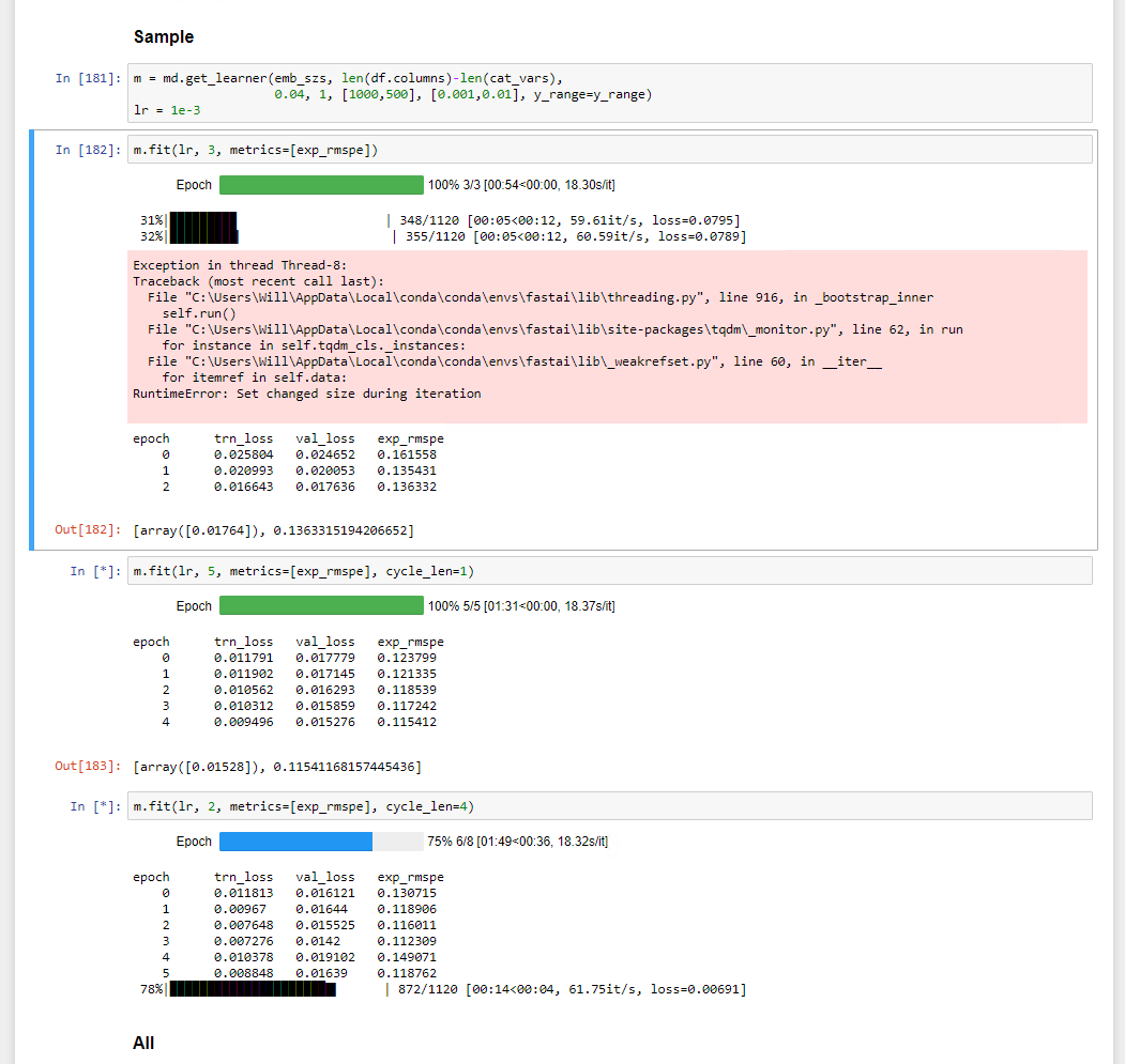
As a side note, I continue to get a strange error when training the sample size network. I get the error and then training continues. This happens every time I run the notebook, haven’t been able to google an answer yet:
Maybe this thread shouldn’t be in the 2017 forum?I
I’m not working on this data set at the moment, but here are a couple ideas:
using denoising auto encoders (DAE), inspired by the winner of the Porto Seguro Kaggle competition. Note that I haven’t seen anyone replicate his solution so far (I am currently trying and haven’t been able so far); so this is not going to be straightforward.
creating another model using LGBM. Tree based algorithms are currently beating NN’s in all the recent tabular data competitions. Would be nice to have a comparison with the Rossman data.