How can both the discriminator loss and generator loss decrease?
The paper uses GANs for super-resolution so it has an extra L1 loss. I do not think that would impact the relationship between the adversarial losses.
real_y = discriminator(real_sample)
fake_y = discriminator(generator(noise))
discriminator_loss = real_y-fake_y+1 # +1 makes it look nicer, between 0 and 2

fake_y = discriminator(generator(noise))
generator_loss = fake_y
I would expect one of the losses to increase as the other one decreases. Since they use the same calculation of fake_y and one decreases -fake_y and the other fake_y. One optimizer is making fake_y less and the other optimizer is making it more.
Maybe the loss functions aren’t calculated like I said.
In the widely used analogy:
In simple terms the generator is like a forger trying to produce some counterfeit material, and the discriminator is like the police trying to detect the forged items.
We can measure how good the police is by how many times out of 100 fakes he can identify the real and fake ones and the forger as deceiving the policeman out of 100 fakes.
Wouldn’t that mean that if the police get better, the forger gets worse? (if using the aforementioned measure of how good they are)
Therefore we wouldn’t be able to see both of them being good at the same time! But the graph from the paper indicates otherwise. I must be missing something!
They both minimize their own loss function. And that doesn’t mean they trade off between each other. Consider an example where the forger makes perfect fakes (its loss=zero), but the discriminator can distinguish between fake and non-fake perfectly ie it’s acc=100% and it’s loss=0
That would be perfect end result towards which gan trainers push, as I understand it.
Let us define perfect fakes as fakes that can fool the discriminator, that are not copies of real samples.
It is then impossible to tell apart perfect fakes and real samples. Unless the discriminator learns all of the real samples but that isn’t what we want (let us say that it didn’t).
Generator Loss 0:
The generator creates perfect fakes all the time, the discriminator is always fooled. The discriminator is fooled meaning it is doing a bad job.
Discriminator Loss 0:
The discriminator is able to tell, all the time, which samples are fake and real. The generator can’t fool the discriminator and therefore is doing a bad job.
These are extremes but one can see how the trade-off would apply in non-extremities too.
I don’t see how there could be no trade-off between the discriminator’s and the generator’s loss. This leads me to not understand how both can decrease at the same time like in the Figure 2 graph.
Ok, fair enough. Let me explain my line of thinking. Suppose generator makes a near perfect bird. There is only 1 pixel ‘off’. So, for this particular example loss is practically zero. At the same time, if discriminator is even more capable, if the discriminator knows even more deeply how the bird should look like, it will detect that there is 1 pixel ‘off’, otherwise it would be perfect indeed.
So it will be marked as fake. Couldn’t that be the case?
Even if the generator makes a near perfect bird, its loss isn’t how perfect the bird is. The generator’s loss is how much it can fool the discriminator. Therefore in the 1 pixel “off” case, the generator’s loss would be very high (because the discriminator was sure that it was fake) even though the generated sample was extremely close to a perfect bird.
you maybe right here, I was just trying to think out loud how it could be explained. Haven’t spent too much time on GANs myself. Just played through some tutorials.
Thanks for helping I am in the middle of training some GANs that is why I am interested. It doesn’t impact the training luckily. I hope someone can answer though. I can’t find many resources on training WGANs unfortunately.
Had to educate myself a little took a glance at the document you referred to.
Found some points that support what I was saying, if I understand correctly.
…
3.3.1 Perceptual Loss
To ensure that the generated images resemble the input image, we require the generator not only
minimize the adversarial loss (JG in Section 3.2) but also the L1 difference between the input image
and the downsized generated image. Hence we define the new generator loss function to be a weighted sum of the above two terms…
…
5.3 Mode collapse
Figure 3(e) and (k) show strong mode collapse with several images being clearly identical, consistent
with existing literature (Goodfellow, 2016 and reference therein). Normally we would not expect to
observe mode collapse in super-resolution images, since they are enforced to look similar to input
files by the L1 loss term in the generator loss (see Section 3.3.1). Their appearance suggests that in
these two examples, the L1 loss term should have a larger weight.
You are right! There is an L1 loss but only for super-resolution. I am speaking of GANs that don’t do super-resolution but turn noise into realistic samples. I should have linked another paper that has an example of those but I couldn’t find one with a graph of generator and discriminator losses.
Thank you for pointing out the L1 loss I will edit the original question.
However, the adversarial loss is the same as in normal GANs. The difference is that L1 loss is being added to it (weighted sum actually). So I still think that having a good discriminator loss would mean bad generator loss even if we add the L1 loss. I still think there is a trade-off in the adversarial losses!
I did not include the graph of the L1 loss because I believe “Generator loss” is not the weighted sum of the L1 and adversarial loss in Figure 2. Because the L1 loss is also plotted in the original Figure 2.
The GAN I am training also displays this relationship between the generator and discriminator loss:
# disc_loss is WGAN-CT loss
# gen_loss output of discriminator when a fake sample is input
# disc_r output of discriminator when a real sample is input
# disc_f output of discriminator when a fake sample is input

 epoch      disc_loss  gen_loss   disc_r     disc_f
    0      -3.379324  0.885375   -3.702462  -0.813928
    1      -3.07398   0.731019   -3.96317   -0.781391
    2      -3.121166  0.364389   -4.529734  -0.299867
    3      -2.89777   0.721051   -4.004071  -0.712604
As the generator gets better at fooling the discriminator (gen_loss decreases) the discriminator becomes worse at telling them apart (disc_f increases). I do not understand why the output of the discriminator is not put in a sigmoid or tanh either.
Oh wow! I understand I think! The output of the “discriminator” in WGANs doesn’t have a sigmoid or tanh activation because it isn’t a classifier! In WGANs the “discriminator” does something else. I will look it up now.
This means that the analogy is incorrect. And I still don’t know what they measured in Figure 2
The paper words it in such a way that I think I might be wrong again…
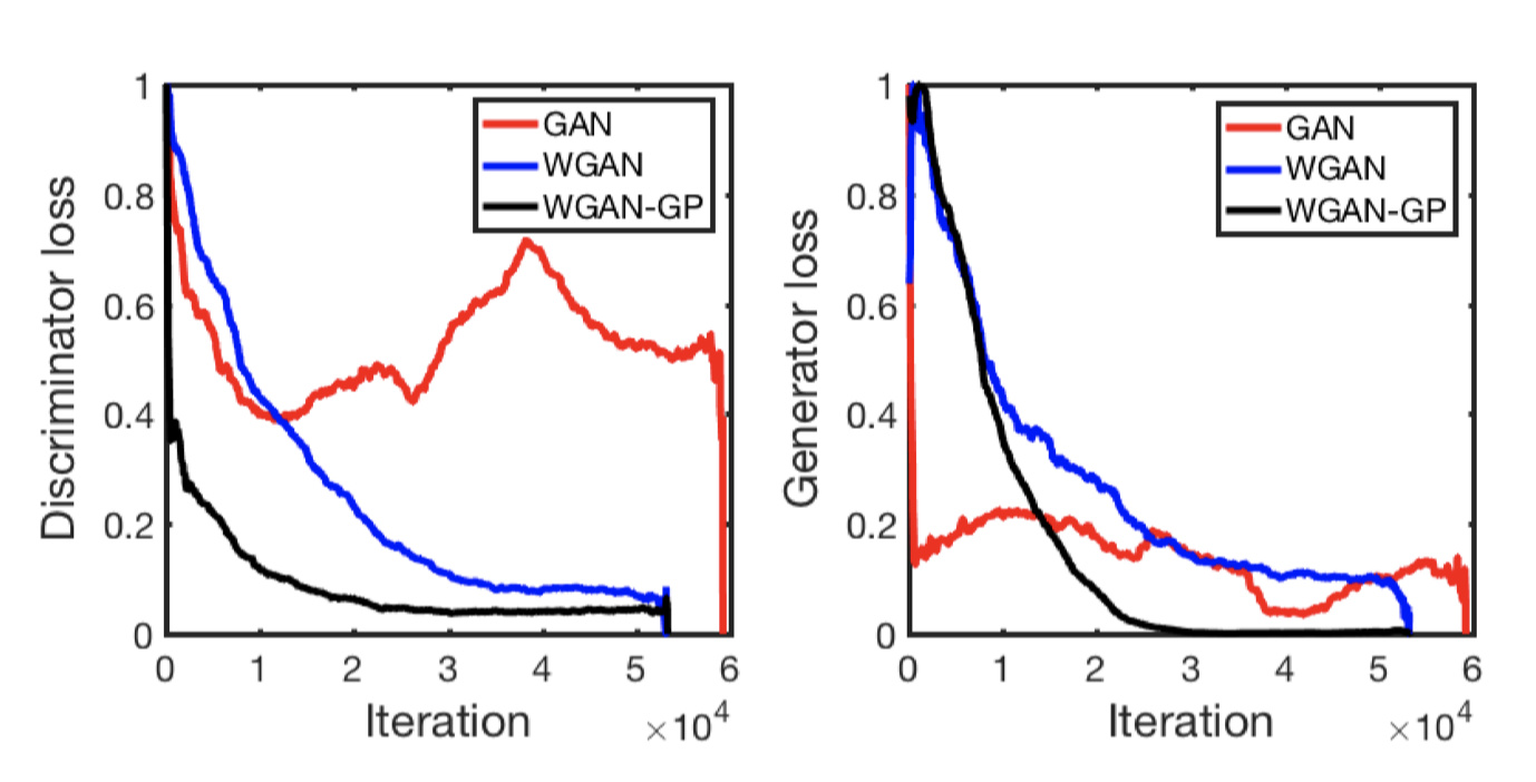
The middle and right panels show the the discriminator loss and generator loss versus training steps. Using WGAN and WGAN-GP objectives, the discriminator loss decreases monotonically, correlating perfectly with training progress, consistent with the claim in Arjovsky et al. (2017b) and Gulrajani et al. (2017). In contrast, the widely used GAN objective leads to oscillating discriminator loss, and therefore does not effectively reflect training progress. We conclude that the WGAN and WGAN-GP objectives honor promises to correlate well with training progress, which is vital for hyperparameter tuning, detecting overfitting or simply deciding when to terminate training.
What is the discriminator loss in WGAN? because it surely isn’t what I am printing
I do print out what my optimizer is minimizing for the discriminator (disc_loss). Same as in WGAN-GP except with an extra consistency term added on.
Thus the “discriminator” is not a direct critic of telling the fake samples apart from the real ones anymore. Instead, it is trained to learn a K-Lipschitz continuous function to help compute Wasserstein distance. As the loss function decreases in the training, the Wasserstein distance gets smaller and the generator model’s output grows closer to the real data distribution.
The loss in WGAN means the distance between the distribution of the data and the generated. So both the generator and the discriminator try to minimize the loss. However, in the loss function,
L = E[D(real)] - E[D(fake)], the previous one has nothing to do with the generator. So when updating generator, we only need to consider the -E[D(fake)].
Minimize E[D(fake)] is the same as minimizing -E[D(fake)].
WGAN employs an art critic instead of a forgery expert.
The critic now is just a function that tries to have (in expectation) low values in the fake data, and high values in the real data. If it can’t, it’s because the two distributions are indeed similar.
I think that what you are missing is that they can both be good at the same time. For example, take the two top soccer teams (or basketball teams, or whatever your favorite sport is). They will play each other, and sometimes one will win, sometimes the other, but each time it is a great match with beautiful action!
However, they are optimizing the same loss function as two mediocre teams.
The training is designed so that each helps the other get better. You are correct that there is a tradeoff between the two, and in the GAN context this tradeoff goes towards what is called a “Nash equilibrium”, which is a mathematical concept coming from game theory.