All,
Apologize for the delay, here’s lecture 3’s notes.
- Tim
Unofficial Deep Learning Lecture 3 Notes
Where do we go from here?
- CNN Image intro ← we are here
- Structured neural net intro
- Language RNN intro
- Collaborative filtering intro
- Collaborative filtering in-depth
- Structured neural net in-depth
- CNN image in depth
- Language RNN in depth
Talking about the Kaggle command line
The unofficial Kaggle CLI tool keeps changing though. So, be careful with different versions.
Use below command to upgrade:
pip install kaggle-cli --upgrade
Note: that the specific name of a Kaggle challenge is listed as follows:
Specific name: planet-understanding-the-amazon-from-space
Don’t forget to enter your password.
curlWget Chrome extension - everytime you try and download something. There’s a yellow button with a command line version to download data. Paste that command in AWS/equivalent console to download data.
%reload_ext autoreload
%autoreload 2
%matplotlib inline
import sys
sys.path.append('/home/paperspace/repos/fastai')
import torch
import fastai
from fastai.imports import *
from fastai.transforms import *
from fastai.conv_learner import *
from fastai.model import *
from fastai.dataset import *
from fastai.sgdr import *
1. Fastai Library Comparison: Short explanation on a quick and dirty Cats vs. Dogs.
Need the following folders:
- Train - with a folder for different
- Valid
- Test
Assuming you download from Kaggle and unzip
from fastai.conv_learner import *
PATH = 'data/dogscats/'
Set image size and batch size
sz = 224; bs = 64
Training a model → straight up
Note: this command will download the ResNet model. May take a few minutes, using ResNet50 to compare to Keras, will take about 10 mins to run afterwards.
By default all the layers frozen except the last few. Note that we need to pass test_name parameter to ImageClassifierData for future predictions.
tfms = tfms_from_model(resnet50, sz, aug_tfms=transforms_side_on, max_zoom=1.1)
data = ImageClassifierData.from_paths(PATH, tfms= tfms, bs=bs, test_name='test1')
learn = ConvLearner.pretrained(resnet50, data )
% time learn.fit( 1e-2, 3, cycle_len=1)

# deeper model like resnet 50
A Jupyter Widget

[ 0.       0.04488  0.02685  0.99072]
[ 1.       0.03443  0.02572  0.99023]
[ 2.       0.04223  0.02662  0.99121]

CPU times: user 4min 16s, sys: 1min 43s, total: 5min 59s
Wall time: 6min 14s
Note: ‘precompute = True’ caches some of the intermediate steps which we do not need to recalculate every time. It uses cached non-augmented activations. That’s why data augmentation doesn’t work with precompute. Having precompute speeds up our work. Jeremy telling this during lecture 3
Unfreeze the layers, apply a learning rate
BN_freeze - if are you using a deep network on a very similar dataset to your target (ours is dogs and cats) - its causing the batch normalization not be updated.
Note: If Images are of size between 200-500px and arch > 34 e.g. resnet50 then add bn_freeze(True)
learn.unfreeze()
learn.bn_freeze(True)
%time learn.fit([1e-5, 1e-4,1e-2], 1, cycle_len=1)
A Jupyter Widget

[ 0.       0.02088  0.02454  0.99072]

CPU times: user 4min 1s, sys: 1min 5s, total: 5min 7s
Wall time: 5min 12s
Get the Predictions and score the model
%time log_preds, y = learn.TTA()
metrics.log_loss(y, np.exp(log_preds)), accuracy(log_preds,y)
CPU times: user 31.9 s, sys: 14 s, total: 45.9 s
Wall time: 56.2 s

(0.016504555816930676, 0.995)
2. Fastai Library Comparison: Keras Sample
Example of running on TensorFlow back-end
To install:
pip install tensorflow-gpu keras
%reload_ext autoreload
%autoreload 2
%matplotlib inline
import numpy as np
from keras.preprocessing
PATH = "data/dogscats/"
sz=224
batch_size=64
import numpy as np
from keras.preprocessing.image import ImageDataGenerator
from keras.preprocessing import image
from keras.layers import Dropout, Flatten, Dense
from keras.applications import ResNet50
from keras.models import Model, Sequential
from keras.layers import Dense, GlobalAveragePooling2D
from keras import backend as K
Set paths
train_data_dir = f'{PATH}train'
validation_data_dir = f'{PATH}valid'
batch_size = 64
1. Define a data generator(s)
- data augmentation do you want to do
- what kind of normalization do we want to do
- create images from directly looking at it
- create a generator - then generate images from a directory
- tell it what image size, whats the mini-batch size you want
- do the same thing for the validation_generator, do it without shuffling, because then you can’t track how well you are doing
train_datagen = ImageDataGenerator(rescale=1. / 255,
    shear_range=0.2, zoom_range=0.2, horizontal_flip=True)

test_datagen = ImageDataGenerator(rescale=1. / 255)

train_generator = train_datagen.flow_from_directory(train_data_dir,
    target_size=(sz, sz),
    batch_size=batch_size, class_mode='binary')

# validation set
validation_generator = test_datagen.flow_from_directory(validation_data_dir,
    shuffle=False,
    target_size=(sz, sz),
    batch_size=batch_size, class_mode='binary')
Note: class_mode=‘categorical’ for multi-class classification
2. Make the Keras model
- ResNet50 was used because Keras didn’t have ResNet34. This is for comparing apples to apples.
- Make base model.
- Make the layers manually which ones you want.
base_model = ResNet50(weights='imagenet', include_top=False)
x = base_model.output
x = GlobalAveragePooling2D()(x)
x = Dense(1024, activation='relu')(x)
predictions = Dense(1, activation='sigmoid')(x)
3. Loop through and freeze the layers you want
- You need to compile the model.
- Pass the type of optimizer, loss, and metrics.
model = Model(inputs=base_model.input, outputs=predictions)
for layer in base_model.layers: layer.trainable = False
model.compile(optimizer='rmsprop', loss='binary_crossentropy', metrics=['accuracy'])
4. Fit
- Keras expects the size per epoch
- How many workers
- Batchsize
%%time
model.fit_generator(train_generator, train_generator.n // batch_size, epochs=3, workers=4,
        validation_data=validation_generator, validation_steps=validation_generator.n // batch_size)
6. We decide to retrain some of the layers,
- loop through and manually set layers to true or false.
split_at = 140
for layer in model.layers[:split_at]: layer.trainable = False
for layer in model.layers[split_at:]: layer.trainable = True
model.compile(optimizer='rmsprop', loss='binary_crossentropy', metrics=['accuracy'])
7. Closing Comments
PyTorch - a little early for mobile deployment.
TensorFlow - do more work with Keras, but can deploy out to other platforms, though you need to do a lot of work to get there.
3. Reviewing Dog breeds as an example to submit to Kaggle
how to make predictions - will use dogs / cats for simplicity. Jeremy uses Dog breeds for walkthrough.
By default, PyTorch gives back the log probability.
log_preds,y = learn.TTA(is_test=True)
probs = np.exp(log_preds)
Note: is_test = True gives predictions on test set rather than validation set.
df = pd.DataFrame(probs)
df.columns = data.classes
df.insert(0,'id', [o[5:-4] for o in data.test_ds.fnames])
Explanation: Insert a new column at position zero named ‘id’. subset and remove first 5 and last 4 letters since we just need ids.
df.head()
| id | cats | dogs | |
|---|---|---|---|
| 0 | /828 | 0.000005 | 0.999994 |
| 1 | /10093 | 0.979626 | 0.013680 |
| 2 | /2205 | 0.999987 | 0.000010 |
| 3 | /11812 | 0.000032 | 0.999559 |
| 4 | /4042 | 0.000090 | 0.999901 |
with large files compression is important to speedup work
SUBM = f'{PATH}sub/'
os.makedirs(SUBM, exist_ok=True)
df.to_csv(f'{SUBM}subm.gz', compression='gzip', index=False)
Gives you back a URL that you can use to download onto your computer. For submissions, or file checking etc.
FileLink(f'{SUBM}subm.gz')
4. What about a single prediction?
assign a single picture
fn = data.val_ds.fnames[0]
fn
'valid/cats/cat.9000.jpg'
can always view the photo
Image.open('data/dogscats/'+fn)
Shortest way to do a single prediction
Make sure you transform the image before submitting to the learn.
im = val_tfms(open_image(PATH+fn)
learn.predict_array(im[none])
(Note the use of open_image instead of Image.open above - this divides by 255 and converts to np.array as is done during training)
Everything passed to or returned from models is assumed to be mini-batch or “tensors” so it should be a 4-d tensor. (#ct, height, weight, channels) This is why we add another dimension via im[none]
trn_tfms, val_tfms = tfms_from_model(resnet50,sz)
Predict dog or cat!
im = val_tfms(open_image('data/dogscats/'+fn))
preds = learn.predict_array(im[None])
np.argmax(preds) # 0 is cat
0
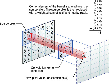
5. Convolution: Whats happening behind the scenes?
Otavio Good’s Video
The theory behind Convolutional Networks, and Otavio Good demo of Word Lens, now part of Google Translate.
The video shows the illustration of the image recognition of a letter A (for classification). Some highlights:
- Positives
- Negatives
- Max Pools
- Another Max Pools
- Finally, we compare it to a template of
A, B, C, D, E, then we get a % probability. - Illustrating a pretrained model.
Spreadsheet Example - Convolution Layers
Definitions
| term | definitions |
|---|---|
| Activations | Input numbers x kernel matrix = numbers |
| Relu | MAX(0, calculated number) |
| Filter / Kernel | refers to the same thing, the 3x3 slice of a tensor |
| tensor | array with more dimensions. In this case, all these filters can be stacked into a multi-dimensional matrix. |
| Hidden Layers | intermediate calculation, not the input, and not the last layer, so called a hidden layer |
| Architecture | how big is your kernel and how many of them do you have ? |
| Name your layers | typically people will name their layers as they create it Conv1, Conv2 |
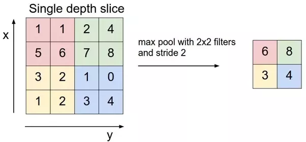
| Max pooling | a (2,2) max pooling will half the resolution in both height and width, as seen in the excel |
| Fully Connected Layer | give every single activation and give them a weight. Then get a sum product of weights times activations. Really big weight matrix (sized as big as the entire import) |
| Note: We do fully connected layer on old architecture or structured data. These days we do can many things after Max pooling. One of them is taking max of Max pooling grid. Architecture that make heavy use of fully connected layers are prone to overfitting and are slower. ResNet, ResNext doesn’t use very large fully connected layers. | |
| activation function | is a function applied to activations. Max ( ) is an example |
Layers
- Input
- Conv1
- Conv2
- Maxpool
- Denseweights
- Dense activation
Example of Max pooling
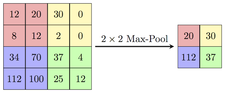
Refer to entropy_example.xlsx.
Now, if we were to predict numbers (0-9) or categorical data… we’ll have that many output by fully connected layer. There is no ReLU after fully connected so we can have negative numbers. We want to convert these numbers into probabilities which are between 0-1 and add to 1. Softmax is an activation function which helps here. An activation function is a function which we apply to activations. We were using ReLU i.e. max(0,x) until now which is also activation function. Such functions are for non-linearity. An activation function takes a number and spits out a single number.
Example of a softmax layer
Only ever occurs in the final layer. Always spits out numbers between 0 and 1. And the numbers added together gives us a total of 1. This isn’t necessary, we COULD tell them to learn a kernel to give probabilities. But if you design your architecture properly, you will build a better model. If you build the model that way, and it iterates with the proper expected output you will save some time.
| output | exp | softmax | |
|---|---|---|---|
| cat | 4.84 | 126.44 | 0.40 |
| dog | 3.98 | 53.60 | 0.17 |
| plane | 4.89 | 132.48 | 0.42 |
| fish | -2.80 | 0.06 | 0.00 |
| building | -1.96 | 0.14 | 0.00 |
| Total | 312.72 | 1.00 | |
| of them |
1. Get rid of negatives
( Exponential column ) - It also accentuates the number and helps us because at the end we want one them with high probability. Softmax picks one of the output with strong probability.
Some basic properties:
$$ ln(xy) = ln(x) +ln(y)  $$
$$ ln(\frac{x}{y}) = ln(x)  - ln(y)  $$
$$ ln(x) = y , e^y = x $$
2. then do the % proportion
$$ \frac{ln(x)}{\sum{ln(x)}} = probability$$
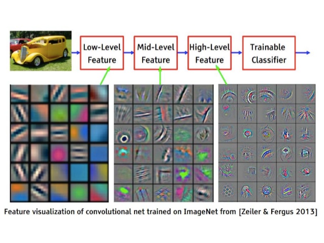
Image models (how do we recognize multiple items?)
import sys
sys.path.append('/home/paperspace/repos/fastai')
import torch
from fastai.imports import *
from fastai.transforms import *
from fastai.conv_learner import *
from fastai.model import *
from fastai.dataset import *
from fastai.sgdr import *
PATH = '/home/paperspace/Desktop/data/Planet: Understanding the Amazon from Space/'
list_paths = [f"{PATH}train-jpg/train_0.jpg", f"{PATH}train-jpg/train_1.jpg"]
titles=["haze primary", "agriculture clear primary water"]
#plots_from_files(list_paths, titles=titles, maintitle="Multi-label classification")
f2 = is f_beta where beta = 2, weights false negatives and false positives much worse
def f2(preds, targs, start=0.17, end=0.24, step=0.01):
    with warnings.catch_warnings():
        warnings.simplefilter("ignore")
        return max([fbeta_score(targs, (preds>th), 2, average='samples')
                    for th in np.arange(start,end,step)])
#from planet import f2

metrics=[f2]
Write any metric you like
Custom metrics from the planet.py file
from fastai.imports import *
from fastai.transforms import *
from fastai.dataset import *
from sklearn.metrics import fbeta_score
import warnings

def f2(preds, targs, start=0.17, end=0.24, step=0.01):
    with warnings.catch_warnings():
        warnings.simplefilter("ignore")
        return max([fbeta_score(targs, (preds>th), 2, average='samples')
                    for th in np.arange(start,end,step)])

def opt_th(preds, targs, start=0.17, end=0.24, step=0.01):
    ths = np.arange(start,end,step)
    idx = np.argmax([fbeta_score(targs, (preds>th), 2, average='samples')
                for th in ths])
    return ths[idx]

def get_data(path, tfms,bs,  n, cv_idx):
    val_idxs = get_cv_idxs(n, cv_idx)
    return ImageClassifierData.from_csv(path, 'train-jpg', f'{path}train_v2.csv', bs, tfms,
                                 suffix='.jpg', val_idxs=val_idxs, test_name='test-jpg')

def get_data_zoom(f_model, path, sz, bs, n, cv_idx):
    tfms = tfms_from_model(f_model, sz, aug_tfms=transforms_top_down, max_zoom=1.05)
    return get_data(path, tfms, bs, n, cv_idx)

def get_data_pad(f_model, path, sz, bs, n, cv_idx):
    transforms_pt = [RandomRotateZoom(9, 0.18, 0.1), RandomLighting(0.05, 0.1), RandomDihedral()]
    tfms = tfms_from_model(f_model, sz, aug_tfms=transforms_pt, pad=sz//12)
    return get_data(path, tfms, bs, n, cv_idx)
f_model = resnet34
label_csv = f'{PATH}train_v2.csv'
n = len(list(open(label_csv)))-1
val_idxs = get_cv_idxs(n)
We use a different set of data augmentations for this dataset - we also allow vertical flips, since we don’t expect vertical orientation of satellite images to change our classifications.
Here we’ll have 8 flips. 90, 180, 270 and 0 degree. and same for the side. We’ll also have some rotation, zooming, contrast and brightness adjustments.
data.val_ds returns single item/image say data.val_ds[0].
data.val_d returns an generator. Which returns mini-batch of items/images. We always get the next mini-batch.
def get_data(sz):
    tfms = tfms_from_model(f_model, sz, aug_tfms=transforms_top_down, max_zoom=1.05)
    return ImageClassifierData.from_csv(PATH, 'train-jpg', label_csv, tfms=tfms,
                    suffix='.jpg', val_idxs=val_idxs, test_name='test-jpg')
PATH = '/home/paperspace/Desktop/data/Planet: Understanding the Amazon from Space/'
os.makedirs('data/planet/models', exist_ok=True)
os.makedirs('cache/planet/tmp', exist_ok=True)
label_csv = f'{PATH}train_v2.csv'
data = get_data(256)
x,y = next(iter(data.val_dl))
y
    1     0     0  ...      0     1     1
    0     0     0  ...      0     0     0
    0     0     0  ...      0     0     0
       ...          ⋱          ...
    0     0     0  ...      0     0     0
    0     0     0  ...      0     0     0
    1     0     0  ...      0     0     0
[torch.FloatTensor of size 64x17]
list(zip(data.classes, y[0]))
[('agriculture', 1.0),
 ('artisinal_mine', 0.0),
 ('bare_ground', 0.0),
 ('blooming', 0.0),
 ('blow_down', 0.0),
 ('clear', 1.0),
 ('cloudy', 0.0),
 ('conventional_mine', 0.0),
 ('cultivation', 0.0),
 ('habitation', 0.0),
 ('haze', 0.0),
 ('partly_cloudy', 0.0),
 ('primary', 1.0),
 ('road', 0.0),
 ('selective_logging', 0.0),
 ('slash_burn', 1.0),
 ('water', 1.0)]
One Hot Encoding:
| Classification | softmax | dog (one-hot) | Index | sigmoid |
|---|---|---|---|---|
| cat | 0 | 0 | 0 | 0.01 |
| dog | 0.92 | 1 | 1 | 0.98 |
| plane | 0 | 0 | 2 | 0.01 |
| fish | 0 | 0 | 3 | 0.0 |
| building | 0.08 | 0 | 4 | 0.07 |
Softmax - probabilities to make 1 choice
one-hot - each column only tracks 1 possible classification. e.g. 3 classes = 3 columns
Index - multi class stored as indices. Taken care of by fastai library.
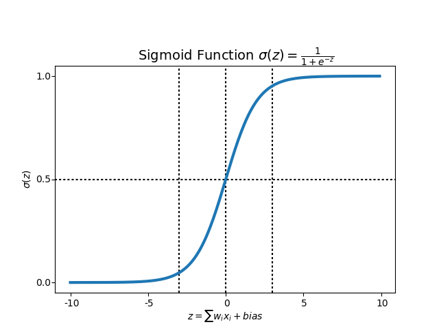
Sigmoid function
$$ = \frac{e^\alpha}{1+e^\alpha}$$
plt.imshow(data.val_ds.denorm(to_np(x))[0]*1.4);
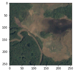
How do we use this?
resize the data from 256 down to 64 x 64.
Wouldn’t do this for cats and dogs, because it starts off nearly perfect. If we resized, we destroy the model. Most ImageNet models are designed around 224 which was close to the normal. In this case, since this is landscape, there isn’t that much of ImageNet that is useful for satellite.
So we will start small
sz=64
data = get_data(sz)
What does resize do?
I will not use images more than image size 1.3, go ahead and make new jpg where the smallest edge is x size. So this will save a lot of time for processing. In general the image resize will take a center crop.
data = data.resize(int(sz*1.3), 'tmp')
Train our model
Note: Training implies improving filters/kernels and weights in Fully connected layers. On the other hand activations are calculated.
learn = ConvLearner.pretrained(f_model, data, metrics=metrics)
To view the model + the layers (only looking at 5)
list(learn.summary().items())[:5]
[('Conv2d-1',
  OrderedDict([('input_shape', [-1, 3, 64, 64]),
               ('output_shape', [-1, 64, 32, 32]),
               ('trainable', False),
               ('nb_params', 9408)])),
 ('BatchNorm2d-2',
  OrderedDict([('input_shape', [-1, 64, 32, 32]),
               ('output_shape', [-1, 64, 32, 32]),
               ('trainable', False),
               ('nb_params', 128)])),
 ('ReLU-3',
  OrderedDict([('input_shape', [-1, 64, 32, 32]),
               ('output_shape', [-1, 64, 32, 32]),
               ('nb_params', 0)])),
 ('MaxPool2d-4',
  OrderedDict([('input_shape', [-1, 64, 32, 32]),
               ('output_shape', [-1, 64, 16, 16]),
               ('nb_params', 0)])),
 ('Conv2d-5',
  OrderedDict([('input_shape', [-1, 64, 16, 16]),
               ('output_shape', [-1, 64, 16, 16]),
               ('trainable', False),
               ('nb_params', 36864)]))]
Search for Learning Rate
lrf=learn.lr_find()
learn.sched.plot()
lr = 0.2
Refit the model
Follow the last few steps on the bottom of the Jupyter notebook.
learn.fit(lr, 3, cycle_len=1, cycle_mult=2)
How are the learning rates spread per layer?
[split halfway, split halfway, always last layer only]
lrs = np.array([lr/9,lr/3,lr])
learn.unfreeze()
learn.fit(lrs, 3, cycle_len=1, cycle_mult=2)
learn.save(f'{sz}')
learn.sched.plot_loss()
Structured Data
Related Kaggle competition: Corporación Favorita Grocery Sales Forecasting | Kaggle
There’s really two types of data. Unstructured and structured data. Structured data - columnar data, columns, etc… Structured data is important in the world, but often ignored by academic people. Will look at the Rossmann stores data.
%matplotlib inline
%reload_ext autoreload
%autoreload 2
from fastai.imports import *
from fastai.torch_imports import *
from fastai.structured import *
from fastai.dataset import *
from fastai.column_data import *
np.set_printoptions(threshold=50, edgeitems=20)

from sklearn_pandas import DataFrameMapper
from sklearn.preprocessing import LabelEncoder, Imputer, StandardScaler
import operator

PATH='/home/paperspace/Desktop/data/rossman/'
test = pd.read_csv(f'{PATH}test.csv', parse_dates=['Date'])
def concat_csvs(dirname):
    path = f'{PATH}{dirname}'
    filenames=glob.glob(f"{path}/*.csv")

    wrote_header = False
    with open(f"{path}.csv","w") as outputfile:
        for filename in filenames:
            name = filename.split(".")[0]
            with open(filename) as f:
                line = f.readline()
                if not wrote_header:
                    wrote_header = True
                    outputfile.write("file,"+line)
                for line in f:
                     outputfile.write(name + "," + line)
                outputfile.write("\n")
Feature Space:
- train: Training set provided by competition
- store: List of stores
- store_states: mapping of store to the German state they are in
- List of German state names
- googletrend: trend of certain google keywords over time, found by users to correlate well with given data
- weather: weather
- test: testing set
table_names = ['train', 'store', 'store_states', 'state_names',
               'googletrend', 'weather', 'test']
We’ll be using the popular data manipulation framework pandas. Among other things, pandas allows you to manipulate tables/data frames in python as one would in a database.
We’re going to go ahead and load all of our CSV’s as data frames into the list tables.
tables = [pd.read_csv(f'{PATH}{fname}.csv', low_memory=False) for fname in table_names]
from IPython.display import HTML
We can use head() to get a quick look at the contents of each table:
- train: Contains store information on a daily basis, tracks things like sales, customers, whether that day was a holiday, etc.
- store: general info about the store including competition, etc.
- store_states: maps store to state it is in
- state_names: Maps state abbreviations to names
- googletrend: trend data for particular week/state
- weather: weather conditions for each state
- test: Same as training table, w/o sales and customers
This is very representative of a typical industry dataset.
The following returns summarized aggregate information to each table across each field.
