Wiki: Lesson 5

Note you’ll need the same fix for subsequent class definitions:

class EmbeddingDotBias(nn.Module):
    def __init__(self, n_users, n_movies):
        super().__init__()
        (self.u, self.m, self.ub, self.mb) = [get_emb(*o) for o in [
            (n_users, n_factors), (n_movies, n_factors), (n_users,1), (n_movies,1)
        ]]
        
    def forward(self, cats, conts):
        users,movies = cats[:,0],cats[:,1]
        um = (self.u(users)* self.m(movies)).sum(1)
        res = um + self.ub(users).squeeze() + self.mb(movies).squeeze()
        res = F.sigmoid(res) * (max_rating-min_rating) + min_rating
        return res.view(res.size()[0],1)

I have a question about using more than 2 features (UserID, MovieID) but also like Movie Genres, etc. Jeremy does mention a hint about it towards the end that we can additionally concatenate latent vectors of movie genres and other features in addition to those of userID, movieID. How do we create those additional latent vectors when collab filtering allows us to crosstab userID against the movieID? If anyone tried this, could you share code please?

Hey could you share your code on how you incorporated an embedding for movie genres??

Thanks.This helped me to run the notebook.
Alternatively we can use res.view(-1,1) as well.

Hello. Could you tell if there’s a mistake in a lecture here: https://youtu.be/J99NV9Cr75I?t=1h23m4s

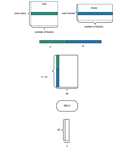
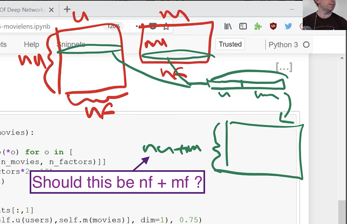
I’m a little confused when Jeremy says that we’re going to multiply our concatenation of user and movie lookups by a matrix that has nu + mu number of rows. My understanding is that it should be nf + mf instead, no? Because when we take extracts from U and M each has a length of nf and mf accordingly and after concatenating them we get nf + mf.

Thanks,
Andrey

yes, I think you are correct. Here is the same diagram re-draw by @hiromi

Just realized this got answered in the previous post. Going to delete.

If anyone is interested, I redid this lesson from scratch here but added a few tweak, such as fitting a model with a learner (so we can use learning rate decay/cosine annealing and reach good score with fewer epochs), clipping output range, using full movielens dataset …

1 Like

what is the intuition behind the above statement, i am having trouble understanding why we would decrease weight decay if there is a lot of variation in the gradient

So in the part of the lecture where we went to excel and did the x,y slope intercept equation learning project, was that a cnn?

Also when we make the crosstab we do:

pd.crosstab(crosstab.userId, crosstab.movieId, crosstab.rating, aggfunc=np.sum)

Why do we need the np.sum? I understand it adds values but what values are there to add? All we are doing is showing what rating a user gave a movie?

I don’t really get the part about adding bias in EmbeddingDotBias class.

My understanding is that in the line:

res = um + self.ub(users).squeeze() + self.mb(movies).squeeze()

um is not a matrix but a vector and squeeze() does not do broadcasting, but removes a dimension of size 1 (bias was a matrix n x 1 so it has to be converted to a vector so it can be added to um).

But in the video it’s said that squeeze() is for broadcasting, which doesn’t make sense to me.

2 Likes

An in-depth but nice explanation of momentum is here: https://distill.pub/2017/momentum/

1 Like

Trying to understand what’s going on here

from sklearn.decomposition import PCA
pca = PCA(n_components=3)
movie_pca = pca.fit(movie_emb.T).components_

Why do we choose to fit the transpose of the movie embedding, rather than the embedding itself? Why do we take the components from the fit PCA rather than transforming the matrix?

I’ve been playing around with different variants and looking at the dimensionality

test1 = pca.fit(movie_emb.T).components_
test1.shape = (3, 3000)

test2 = pca.fit(movie_emb).components_
test2.shape = (3, 50)

test3 = pca.fit_transform(movie_emb)
test3.shape = (3000, 3)

If someone can illuminate what’s going on here and why we use pca the way we do, I would appreciate it.

I was just reviewing this today and wondering the same thing.

In the Lesson 4 notebook, the transposition gives us (features, examples) … but when I look at the docs, the format to be applied should be (n_samples, n_features).

Given this, I’m inclined to think the notebook is wrong here and that it should be:

movie_pca = pca.fit_transform(movie_emb) # returns a (3000,3) matrix

See also here where indeed the dimensionality is reduced from 64 to 3 with the shape as stated per the docs.

If I’m missing something, would love to hear what it is :slight_smile:

Scratch everything I said above.

I’m keeping my post above so folks that are similarly confused by similarly thinking about PCA as I was, can see where I went wrong with my assumptions of how it worked. I spent this past weekend really digging into PCA … how it works, where it is useful, and to what objectives it can be applied too. I include a list of resources below that I found helpful, but let’s get to answering your two questions first:

Why do we choose to fit the transpose of the movie embedding rather than the embedding itself?

The answer lies in part by asking ourselves two questions:

  1. "What does the data represent?
  2. “What is the problem we are attempting to solve?”

The answer to the first question is that our (3000, 50) matrix represents 3,000 movie reviews by 50 things the model has learned about movie reviews that make them meaningful for language modeling and classification. We don’t know what each of these 50 embedding values represent, but we do know that whatever they are, they provide a good representation of each movie review because they have proven useful in the classification task.

The answer to the second question is that we are trying to reduce these 50 things to 3 things and then figure out how related each of the 3k movie reviews are to each of these 3 things so we can infer what the 3 things represent. We are asking, “How can we cluster these 50 different things learned into 3 big areas?” (Notice that we are NOT trying to reduce the dimensionality of each movie review. If we were, we wouldn’t want to transpose the embedding matrix and we wouldn’t care about the components.)

So …

By transposing the matrix so that are examples become the 50 things each of our embeddings have learned about the movie reviews and the features become the 3k movie reviews, when we call pca.fit(movie_emb.T), we are asking PCA to essentially figure out how much each review plays a part in each of the 3 learned principal components. That is exactly what we want!

Why do we take the components from the fit PCA rather than transforming the matrix?

Because they represent the eigenvector for each principal component.

What is an ‘eigenvector’ and why do we care about this?

Simply put, the eigenvector represents how many parts each feature (the 3k reviews) plays in composing the PC. The higher the number, the more important the review is for that PC, and therefore, the more representative of what the PC means.

So look at the dimension of .components_ and you’ll notice that it is (3,3000). The first row is the eigenvector for PC 1 … and each value in there tells you much each review played a part in learning that PC. Thus, if you order the reviews in the first row in descending order, you will have those that are most strongly correlated to PC 1. That information can then be used in turn to infer what PC 1 means.

Grab a cold one and think on all this and I guarantee it will start to make sense

Helpful resources:
2 Likes

I have a question about Pytorch’s RNN segment. When we are doing the manual version, for concatenation, we just create a linear layer of n_fac + n_hidden and do a torch.cat operation of the embedding of the input like so inp = torch.cat((h, self.e(c)), dim=1).

I would like to do something similar using the Pytorch’s RNN module. I created an RNN layer of dimension self.rnn = nn.RNN(n_fac + n_hidden, n_hidden). But I’m not sure how to match the dimension during concatenation as the hidden state is a rank 3 tensor. Any ideas?

This was helpful in wrapping my head around things. I get what’s going on with the linear algebra now.

I’m still left with the question of why we used PCA in this particular fashion instead of using it to reduce the matrix weights into 3 dimensions and plotting those.

I did a quick notebook looking at each method. The clustering results, while not identical, are very very similar. So I guess this is one of those things where it doesn’t really matter either way?

I was able to figure out how to do it. I’m posting it here in case others are looking for it and to see if anyone else has it done in a more efficient way.

Here is the module:

class CharConcatRNN(nn.Module):
    def __init__(self, vocab_size, n_hidden, n_fac):
        super().__init__()
        self.e = nn.Embedding(vocab_size, n_fac)
        self.rnn = nn.RNN(n_fac + n_hidden, n_hidden)
        self.l_out = nn.Linear(n_hidden, vocab_size)
    
    def forward(self, cs):
        bs = cs.shape[0]
        cs = cs.transpose(0, 1).contiguous()        
        h = cs.new_zeros((1,bs,n_hidden), dtype=torch.float)
        expand_h = [cs.shape[0] // h.shape[0]] + [-1] * (len(h.shape) - 1)
        inp = torch.cat((self.e(cs), h.expand(*expand_h)), dim=-1)
        outp, h = self.rnn(inp, h)
    
    return F.log_softmax(self.l_out(outp[-1]), dim=-1)

This is using Pytorch 0.4. There are 3 lines of code here that are important.

  1. The key is to manually broadcast the h tensor to match the shape of self.e(cs) so that we can concatenate it on the 3rd dimension (which means the other two dimensions have to match). I got this trick from this stackoverflow question.
  2. In order to do the manual broadcasting, I had to transpose the first two dimensions of cs (whose code I copied from the custom loss function nll_seq_loss
  3. I used the method new_zeros to initialize h.(documentation here). According to the documentation, the new zero-valued tensor is put on the same device as the source, which means if the module resides on the GPU h will get initialized on the GPU (similarly for the CPU). If we use just torch.zeros we would have to add .cuda() to it to get it on the GPU.

Thanks.

They are related but not the same thing.

The eigenvector for each PC is what tells us how important each feature is to the PC, and what we are particularly interested to know is which reviews are more important for each PC. This vector is made available to us via the .components_ property.

So consider what happens when run this code:

pca.fit(movie_emb)
x = pca.transform(movie_emb)
eigens = pca.components_

x is a (3000,3) dimensional matrix where each value represents the transformed “embedding” value required to reduce the dimensionality of the data form 50 to 3. The eigens is a (3,50) dimensional matrix and tells us how important each embedding column is to each of the 3 principal components.

But we aren’t interested in ranking the importance of the 50 embedding columns to each PC … we want to rank the importance of each movie reviews with respect to each PC

Consider this now …

pca.fit(movie_emb.T)
x = pca.transform(movie_emb.T)
eigens = pca.components_

x is a (50,3) dimensional matrix where each value represents the transformed “movie review” value required to reduce the dimensionality from 3000 to 3. The eigens is a (3,3000) dimensional matrix and tells us how important each movie review is to each of the principal components.

That is what we want.

If we simply wanted to project the 3,000 reviews into a 3-dimensional space, then simply using x from the first approach would be sufficient. But as we are here interested in how important each movie review is to each PC, the latter approach seems correct.

See also:

TL;DR Using approach #2, we are reducing the dimensionality of the 3000 reviews to 3 and then using the .components_ property to find out how important each of the 3000 movie reviews are to each PC

1 Like