Hi, I’m looking for some pointers on describing the default architecture used by fastai tabular. I’m trying to explain this in understandable terms for the methods section of a statistical report. I’ve written the following so far. Very messy and confusing so far.
I’m skipping explaining the way input data is treated with embedding layers, etc to keep it short.
Deep Learning is a subfield of machine learning concerned with algorithms inspired by the structure and function of the brain called artificial neural networks. Neural networks employ the back-propagation algorithm to calculate optimum weights to predict the output class (Equation 1). The output of a single neuron is defined as a^{l}_{j} of j^{th} row and l^{th} layer, where w^{l} are weights connected to the l^{th} layer of neurons and sum is over all k neurons in the (l-1)^{th} layer. The aim is to find weights, which ensure that for each input the output produced by the network is the same as the desired output vector. To minimise the error, gradient methods are used, and the errors are back propagated through the network.
Equation 1:
a^{l}_{j} = \sigma (\sum\limits_{k} w_{jk}^{l} a_{k}^{l-1} + b_{j}^{l})We decided to implement a deep learning model using fastai (version: 2.0.16) with a PyTorch backend (version: 1.6.0) in Python (version: 3.8.6). The fastai library provides quick access to deep learning model building, training and evaluation for vision, text and tabular data. We decided to use its default architecture and parameters for tabular data to develop our prediction model.
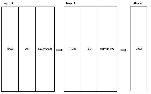
Figure 1 gives a high-level visualization of the architecture for the proposed methodology. The data enters the network through an input layer and then passes through Layer 1, a 200-node hidden layer. A linear transformation is applied to obtain a linear combination (matrix multiplication) of the inputs and the connection weights between the nodes of the input layer and Layer 1. The linear combination also includes a vector addition of bias terms associated with each node of Layer 1. These bias terms are determined by an external bias node providing a bias input to each node of Layer 1, which each node can weight independently to achieve the effect of a translation vector. Next, to introduce non-linearity, the linear combination of each node runs through a Rectified Linear Unit (ReLU) function (Equation 2).
Equation 2:
f(x) = max(0,x)Finally, we normalize the output of Layer 1 by adjusting and scaling the results of the ReLU function for the entire layer (batch normalization). The transformed data then feeds forward into a 100-node hidden layer (Layer 2), which repeats the same steps as Layer 1. The output from Layer 2 feeds forward into the output layer, where a linear transformation of the data allows the network to make the final prediction probabilities for the different classes. The predicted probabilities (\hat{y}) are then compared with the true outcome (y) using cross entropy loss (Equation 3). Cross-entropy loss increases as the predicted probability diverges from the actual label.
Equation 3:
Loss = -y . log(\hat{y})Based on the output of the loss function, the network will then aim to minimize the loss by adjusting the network’s weights and biases of the different layers using backpropagation. Backpropagation computes gradients (partial derivatives) of the loss function and makes use of stochastic gradient descent to find optimal weights and biases to minimize the loss.
Figure 1:
