The history of our field and some of the basic intuitions behind it really are quite extraordinary. And, as you allude to, the mysteries and beauties (really, very profound beauties) are a real joy and challenge as the journey progresses.
So this thresholding is what contributes to the property of “Universal Approximation” - that says simple neural nets can approximate continous functions.
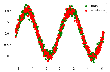
For example take a simple dataset exhibiting a sine wave:
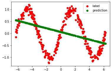
A simple (2 hidden layer) neural network without thresholding cannot approximate this function:
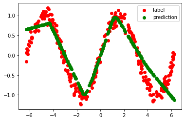
However, if we introduce the thresholding (ReLU) between the 2 layers, the same network can magically learn to predict (approximately) as per the sine wave function:
P.S: The code uses concepts which you will learning in upcoming lessons, but if you are adventurous you can check it out.
In my understanding, this is implying that he’s talking about a ReLU type of an activation function which essentially is “replacing negatives with zeroes”.
Also there’s a lot to unpack in that one sentence. “Multiplying things together” refers to w1 * x1 … wn * xn operation (multiply each input with its respective weight) and adding refers to where we simulate the “integrative behavior” of a so called biological neuron. We just add all these inputs which have now been modified to reflect the strength of each incoming connection (via the multiplication by weight operation) and that is what the activation function gets as its input.
A biological neuron doesn’t control the strength of each incoming dendrite (at the tactical level) so it is only concerned with whatever signal is being pumped in via any given synapse, and then a spike occurs when the sum total of all inputs makes the internal potential go over “a threshold” (not sure what it is tbh… maybe like -70 microvolts or something like that?)
But in our ANNs we calculate the strength of each connection by multiplying each input with its strength (or weight) and THEN add them up (which is the key part actually). In biological neurons the strength of each neuron is in the synapse or number of synapses and how much signal each “pre synaptic neuron” sends forward to us. In an artificial neuron (or node) need to encapsulate that synaptic process in the “multiplication” piece to account for the “strength” of each incoming input, and the back propagation basically adjusts these strengths.
All the various ‘activation’ functions in these artificially simulated nodes try to capture that process (in my limited understanding)
Neural Networks is a mathematical function that takes inputs and multiplies them together by one set of weights and adds them up and dose that again for a second set of weights and then take all the negative numbers and replaces them with zeros, and then take those as inputs to the second layer and do the same thing multiply them and adds them up and dose that a few times.
The Questions are:
1- Is the number of sets of weights must be (or are) an exact match to the number of batches from the input dataset?
2- if the answer to question 1 is “No”, is the number of sets of weights a variable that the model designer can self-set as see fit?
3- why Jeremy says sets of weights?, did he means that the weights go to the model in batches like the input dataset?
@falmerbid, Its 30 years since my brief undergrad encounter with neural nets, so this may be wrong (and when I’m corrected I’ll have learnt something) - but I understood this to mean…
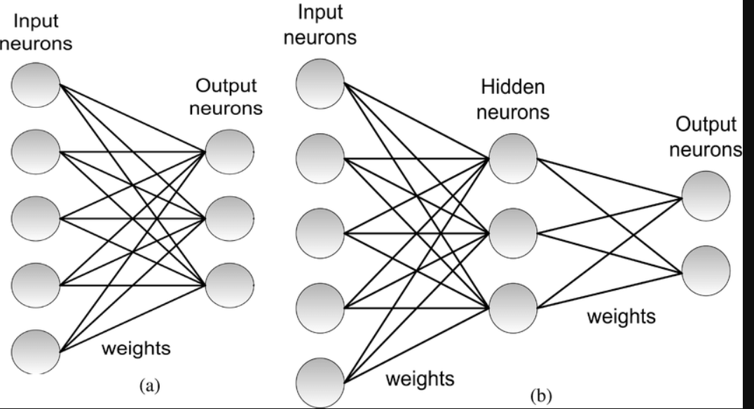
“Each set of weights is a layer in the neural net.”
your answer sounds correct but it doesn’t match Jeremy illustration that I have provided in my question above.
as per my understanding from Jeremy, for each layer we multiply and sum up inputs by multiple sets of weights then we take the result from all of that multiplication and summation as input for the next layer.
I think you and me would like another opinion or more clarity on my question.
I’ve noticed that whenever you train for a single epoch, several things happen underneath the cell.
Training runs for a single epoch to fit / connect the head of the pre-trained model to our new random head for the purposes of whatever we’re doing
Then it trains again for a single epoch (as specified), updating as per our training data.
But for each epoch, it seems like there are two separate stages. One is slow (what I think of in my head as the ‘real training’) where the progress bar completes one cycle of 0-100% and then it again goes through the progress bar from 0-100% quite a bit faster.
What are those two separate processes going on underneath? (Possible we might find out about those at a later stage, in which case feel free to tell me just to wait until a later lesson ) Should I think of them as two separate processes? Is it some kind of consolidation or calculation that’s being represented there?
I think the first slow step is the ‘real training’ of updating the parameters on the training data, and the second fast step is calculating the metrics on the validation set (with the now updated weights).
Off the top of my head, I believe you’re talking about the different progress bars of training phase followed by a validation phase (on the separately held out validation data).
Jeremy will definitely get into more details about these in the upcoming lectures.
I wondered about that too. I sort of figured the general idea as you describe but would be good to know about the two stages during the second epoch , maybe there’s a way to make the output more verbose (or maybe not.)
EDIT: I’m not sure if I’m looking in the right place but looks like the progress callbacks has some details on what might be happening behind the scenes:
From the docstring:
_docs = dict(before_fit="Setup the master bar over the epochs",
                 before_epoch="Update the master bar",
                 before_train="Launch a progress bar over the training dataloader",
                 before_validate="Launch a progress bar over the validation dataloader",
                 after_train="Close the progress bar over the training dataloader",
                 after_validate="Close the progress bar over the validation dataloader",
                 after_batch="Update the current progress bar",
                 after_fit="Close the master bar")
I’m not sure if there is a way to make the progress bars “announce” what they’re doing so to speak , ie print out which call back is being called etc.
Why do we choose error rate instead of accuracy when we’re training our model? Is it a tradition or just something that people do? Accuracy seems more intuitive to me somehow…
One book that I found helpful was Andrew Glassner’s “Deep Learning, A visual Approach”. It is not math heavy at all and a beautifully illustrated book. The title picture is rather drab which is unfortunate, because the book is really geared towards beginners and tries to explain a lot of concepts visually.
Andrew Glassner gave a lecture for non practitioners as well which some might find helpful in grokking the basic concepts of SGD and neural networks without all the intimidating math parts.
Just looked at the PDF and this looks great. I love visual illustrations, when done right it can be very ‘obvious’ and help in explaining complex concepts. I might get a paper copy of this book just for the sake of illustrations. Thanks for sharing !
Yeah, it’s unfortunate the book’s cover is not attractive at all! I almost skipped over it while browsing through books at the library, but when I looked at the illustrations, I checked it out. I’m thinking of getting a copy too because I had to return it and now I’m in the hold queue again
It is printed on thick paper so the book is quite hefty, but YMMV.
Jeremy graciously showed how an SGD version via Excel, which helped clear out a few things. Seeing the whole process of multiplying and summing was beneficial. I still have a few questions:
If we were to visualize the NN he showed, it only has an input of (1424,10), a weight matrix of (10,2), and then an output of (1424,2), correct? To be clear - this is a one-layer NN, with no hidden layer: x_1, … x_m as an input (+bias), multiplied by the weight matrix, and then we’re getting only z_1, z_2 (for a single passenger – Lin1, Lin2). Is this true?
Why did we add up the two ReLUs? assuming we applied a nonlinearity on z_1 and z_2, why do we add these two?
When he refers to GPU and how it’s easier to parallelize these calculations, we can only compute one layer at a time, correct? cause we do need the output on one layer before we continue to the next layer (which we didn’t see in his example if I’m not mistaken).
 ) Should I think of them as two separate processes? Is it some kind of consolidation or calculation that’s being represented there?
 | SIGGRAPH Courses")