Hi all…
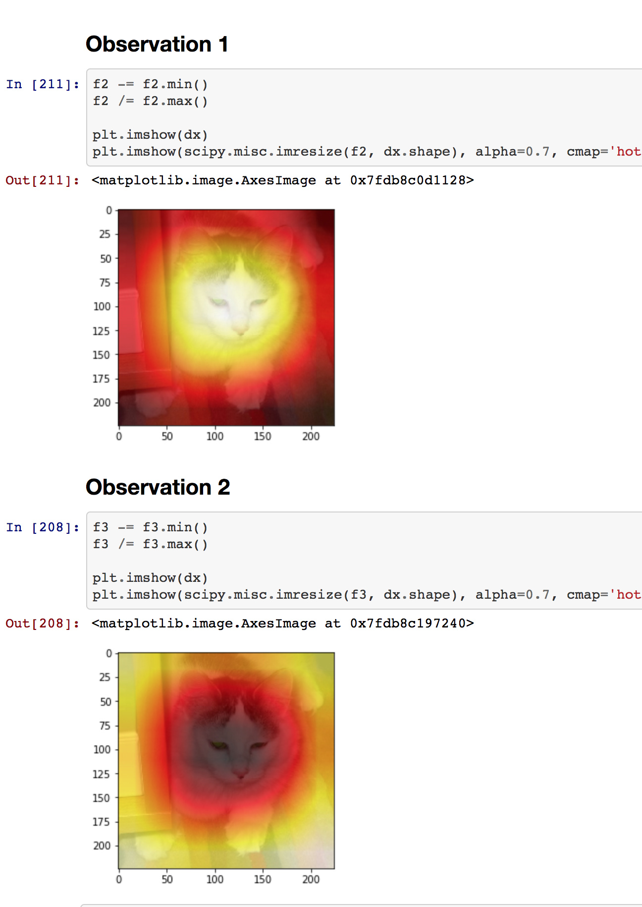
So briefly experimented with the heat-map generation notebook, and here’s something interesting (or maybe uninteresting) I found out. If we take feat, and instead dot.product with array([0., 1.]), then we get a heat-map that is like the reverse of taking the dot.product with array([1., 0.]).
Please find this in here (link to notebook)
Notice how f3 is defined as the follows:
f3 = np.dot(moved, np.array([0., 1.]))
versus how f2 is originally defined as:
f2 = np.dot(moved, np.array([1.0, 0.]))
Also, notice that I didn’t rescale feat which was lower_bounded by 0 originally.
i.e. instead of having
feat = np.maximum(0,sf.features[0])
i simply have now:
feat = sf.features[0]
The differences in the heat-map for f2 and f3 are quite similar, except for the magnitude which is completely flipped.
Just thought it was interesting in that both the two filters from the last convolution layers actually held substantial information. @jeremy Any intuition why it is that we see this?
