At the end of Lesson 5 we learned that collaborative filtering can approximate the results of a user - movie rating database with astonishingly low error. But this seems to be a dead end – all we’ve really done is reproduce the results of a giant movie rating survey – we haven’t gained any new knowledge.
For our result to be practical, we would want to be able to predict how a new user who is not in our database would rate a new movie that is not in our database.
How could we do this? If the user and movie embeddings were based on a set of features, we could compare their embeddings to their nearest neighbors in the training set and use some sort of averaging to predict how any new user would rank any new movie. But there aren’t enough user and movie features.
So I am a bit perplexed here as to how these results can be used practically. Can anyone weigh in with some additional insight?
Just for fun, I modified the EmbeddingNet class to incorporate an embedding for movie genres. As Jeremy predicted, this didn’t improve the score.
I think the really amazing takeaway from this part of Lesson 5 is the simplicity of the matrix factorization technique that allows us to decompose a huge MxN rectangular matrix into the product of an MxJ matrix and a JxN matrix, for arbitrary integer J! This means solving for M*N*J^2 weights given only M*N datapoints!
I did watch again the video of the lesson 5 (part 1) to get the whole image and I took notes of the vocabulary used by @jeremy.
Let’s play ! OK ?
Can you give a definition / a url / an explanation for all the followings terms and expressions ?
If yes, you are done with the 5th lesson !!!
PS : you do not want to test yourself or you want to check your answers ? Go to the blog post “Deep Learning 2: Part 1 Lesson 5” of @hiromi : " super travail !!! "
Structured Deep Learning : not a lot of paper on Deep Learning for structured data with comparaison to computer visionand language natural
this course starts the 2nd half of parte 1 (let’s dive into the source code) : the first half was about understanding the concepts, knowing best pratices and running the code by going through aplications (notebooks); this one is about the code to write with a high level of description
Goal of the lesson : create a collaborative filtering model from scratch (notebook : lesson5-movielens.ipynb)
Movielens dataset is a list of ratings
we use userid and movieid (categorical variables) and rating (independant variable) (we do not use here timestamp)
we get the users that watch the most movies and the movies most watched
in the beginning of the course, we are not going to build a Neural Network but a collaborative filtering model.
we use pandas in the jupyter notebook in order to create a crosstab table of the 15 users they give the most ratings vs the movies which were the most rated
Then, we copy/call this table of numbers atuais in Excel.
** functions to know : pd.read_csv, groupby(), sort_values(), join, crosstab()
** We copy/paste the stucture of the table and put ratings numbers by random (how ? each rating is the dot product of 2 vectors : one that qualifies a user and the other that qualifies a movie. The initial values of these 2 vectores are taken by random. When there is not a true rating, we put zero as the prevision).
** Then, we create an error cell that computes the root-mean-square error (RMSE) which is square root of the mean of the error square).
** This is not a neural net but a single matrix multiplication between 2 matrixes (one of the users and one of the movies)
** In Excel, we can do Gradient Descent : go to Data >> Solver >> Objective function (the cell with the RMSE) : cells to change + MIN (using GRG NonLinear which is Gradient Descent method)
** As this is not a Deep Neural Network (there is no hidden layer), we call this shallow learning.
** We do here a matrix decomposition (probabilistic matrix factorization)
** The numbers for each movie and for each user are called latent factors do vector de embeddings. The gradient descent tries to find these numbers.
** how do decide the dimensionality of our embedding matrix ? No idea. We have to try things and this have to represent the true complexity of the system but not too big (avoid overfitting, avoid time consuming for computation)
** the negative value in the embedding matrix represents the oposite (ie, I do not like)
** if you have a new user, you must retrain your model but we will see that later
Back to the jupyter notebook
** we use get_cv_idxs() to get our validation set
** wd means weight decay (L2 regularisation)
** n_factores : size of our embedding matrix
** our data model is cf = CollabFilterDataset.from_csv()
** our learn model is learn = cf.get_learner() with an optimizer which is optim.Adam
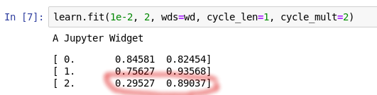
** learn.fit(lr, wd=wd, cycle_len = 1, cycle_mult=2)
** the error is the MSE (mean squared error), not the RMSE, then we need to take the root
** that’s all : the fastai library allows us to get a better validation loss in 3 lines of codes (cf, learn, learn.fit) than the actual benchmark
** Let’s try now to build the Collaborative Filtering from scratch using pytorch
** we can create a torch Tensor in pytorch by using capital T : T([1.,2],[3, 4])
** The multiplication of 2 torch Tensor is a element wise multiplication
we are going to build a layer (our custom neural net layer or custom pytorch layer) = a pytorch module
** And then we can instantiate a model as a pytorch module, use it as a function that we can compose with very conveniently (take the derivative for example)
** to create a pytorch module, we need first to create a pytorch class in which you return the calculated value in a special method called forward
** in a neural net, when you calculate the next activations, it is called the forward pass : it is doing a forward calculation (the gradient is called the backward calculation but we do not have to define that as pytorch does it automatically)
** first thing to do is to get a continuous index of userid and movieid to avoid a huge embedding matrix (we use for that the unique() method and the creation of dictionary)
** each time we want to pass our new number of users, movies (we call them states), we need a constructor for our class (this is a special method def __init__)
** 2 other things to get a full pytorch layer : we inherit of the nn.Module class to get all cool staff from pytorch and we need to call the super class constructor (when we create our own constructor : super().__init__())
Then, we need to give some behavior and we do that by storing somethings in it.
** we create self.u which is an embedding layer : self.u = nn.Embedding(n_users,n_factors), same thing with movies
** we need now to initialize by random our embedding matrices but with small numbers
** the embedding matrix is not a tensor, it is a variable (a variable is a tensor and it does automatic diferentiation)
** then to get the tensor, we use the data attribute
** uniform_ does operate in the same tensor (fill in the matrix)
** finally, we create the forward method by grabbing the embeddings vector for the user and the movie (minibatch of them : this is done autmatically by pytorch : DON’T DO A FOR LOOP because it does not use GPU), and return the dot vector multiplication
** Then, we can write our 3 lines of codes : data with the fastai library, our pytorch module (our model) that we initiate with our EmbeddingDot class, and finally we can fit our model by using the pytorch way
Biais
** we need to add a constant for each user and one for each movie to take account the fact that for example the user always gives a high rating and that a movie is liked by everyone because these are biais : they hide the true diferences.
** Then, we modificate our pytorch module to take account the biais.
** we use broadcasting to add a matrix and a vector (squeeze())
** then, we use a sigmoid function to put all calculations between 1 and 5 (it is not common but help)
** all the functions in pytorch are availables in capital F (F.sigmoid)
** we must precise cuda() as we don’t use a learner from fastai
** One remark : we do not do exactly matrix factorization
** before the Netflix prize, this matrix factorization had actually already been invented but nobody noticed and in the first year of the Netflix price, someone wrote this really famous blog post where they basically said “eh just use it” (2009 by BellKor’s Pragmatic Chaos team)
let’s create a neural net version of this
** A one embedding is exactly the same as doing a one hot encoding.
** An embedding is a matrix product
** the only reason it exists, it is because it is an optimization : it is a computational performance thing for a particular kind of matrix multiplier
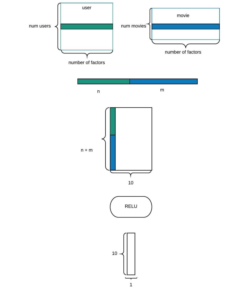
** Our neural net will take in the entry a concatenation of the 2 embeddings vectores : this is an embedding net
** We start with 2 linear layers (then the first one is an hidden layer) and the second one has only one output as we want a single number (we use nn.Linear()). These layers are Fully Connected Layers.
** In the forward method, we grab the data (users and movies) and create the embeddings vectors, we concatenate theses vectors with torch.cat(), we add dropout, we add relu on activations of the layer 1 (F.relu), and activation function after the layer 2 (F.sigmoid())
** Then, we create our data model, our learn object and we fit this learn object with the MSE function (F.mse_loss)
** Point important : we do not need to get the same size of latent factors in the embeddings vetores of user and movie (for example, the embedding vector of the movies can have latent factors for genre and duration for example besides the n_factors shared with the user embedding vector)
Let’s use graddesc.xlsm to implement Gradient descent in excel
** errb1 : finding the derivative through fine diferencing
** derivative of the cost function is how the dependent variable (loss function) changes when the independant variable (intercept or slope) changes
** Jacobian and Hessian matrix
** Chain rule
** mini batch de size 1 = online gradient descent
** problem : it takes time and more, we can see that the error function goes down the same way : it means we can go faster. This is momentum
momemtum is a linear interpoletion between our derivative of the error function (small number) and the ones calculated before : keep doing the way we did before and upgrade a little bit
** everyone uses momentum
** More one point : in momemtum, the learning rate does not change
Adam
** We use SGD with momentum by default in the fastai library but we can now use Adam with weight decay in Fastai (Adam-W)
** Adam has 2 parts : one uses the momemtum of the gradient and the other part uses the momentum of the gradient square
** we use a lot the linear interpolation in DL papers
** if there is a lot of variance of the gradients, the number that divises the learning rate (the square root of the moving average of our squared gradient) will be high and than, the learning rate general is low
** ADAM is finally an adaptative learning rate (but there is only one learning rate)
L2 or weight decay
** when you have huge neural network, lots of parameters, more parameters than data points : then, regularization is important (like dropout)
** we take our loss function and add an aditional piece to that (square of the weights)
** the loss function wants to get the weights small
** if you have a huge weight decay, the gradient descent will keep your parameters to zero : it will never overfit
** if you then decrease the weight decay, some parameters will rise but the ones useless will stay to zero (proche de zero)
** when there are a lot of variation, we end up decreasing the amount of weight decay (and the oposite is true)
ADAMW
** penalize paremeters with weight very high unless their gradient varies a lot : but we do not want that
** so in ADAMW we do not mix weight decay with ADAM
** majority of models uses dropout and weight decay
I am trying to understand the arithmetic behind the choice of weight initialization that Jeremy uses (around the 47 minute mark). He uses a uniform random variable on [0,.05]. What is the arithmetic to arrive at that number? It seems to me that, for example, the maximum of the interval should be weight s.t. max score = (weight^2)*num_factors since that is the dot product of the embedding matrices. What am I missing?
I recreated the whole thing in Keras and found that embeddings are, in fact, meaningful (but their meaning is not immediately obvious). With 100-dim embeddings, here’s how kNN search works for me:
## find similar to Golden Eye movie_emb.iloc[similar50([10], 20)[0], :4]
	movieId	title	genres	bias
      9	10	        GoldenEye (1995)	Action|Adventure|Thriller	0.221678
1273	1722	Tomorrow Never Dies (1997)	Action|Romance|Thriller	0.170194
2272	2990	Licence to Kill (1989)	Action	0.018498
2271	2989	For Your Eyes Only (1981)	Action	0.096108
2345	3082	World Is Not Enough, The (1999)	Action|Thriller	0.248690
2757	3639	Man with the Golden Gun, The (1974)	Action	0.219623
1774	2376	View to a Kill, A (1985)	Action	0.117994
1241	1672	Rainmaker, The (1997)	Drama	0.263498
1577	2115	Indiana Jones and the Temple of Doom (1984)	Action|Adventure	0.381587
1512	2045	Far Off Place, A (1993)	Adventure|Children's|Drama|Romance	0.076758
1059	1401	Ghosts of Mississippi (1996)	Drama	0.198065
1861	2470	Crocodile Dundee (1986)	Adventure|Comedy	0.257988
334	 408	        8 Seconds (1994)	Drama	0.056840
2607	3441	Red Dawn (1984)	Action|War	0.228135
1037	1375	Star Trek III: The Search for Spock (1984)	Action|Adventure|Sci-Fi	0.165070
2275	2993	Thunderball (1965)	Action	0.169414
2756	3638	Moonraker (1979)	Action|Romance|Sci-Fi	0.147252
2196	2889	Mystery, Alaska (1999)	Comedy	0.302645
2755	3635	Spy Who Loved Me, The (1977)	Action	0.193987
208	257	Just Cause (1995)	Mystery|Thriller	-0.069102
While watching a lecture I spotted that the results of fitting models (fastai first model, dot product model, and mini net model) are overfitted. For instance:
As I understand, generally we want to keep train and validation losses close to each other. So my question is
why we let them differ here and at which situations can we let them differ, and by how much? Thanks!
What does those validation indexes suppose to mean in Collaborative filtering context? Does one index mean we will predict the rating for all the movies of that particular user?
In classification or regression cases for structured data set, a data point in validation set means we’ll predict a particular number for that data point. Now sure how that would work in this scenario.
Any help would be appreciated.
Collaborative Filtering from Scratch: Runtime Error during fit. (line 41)
“RuntimeError: input and target shapes do not match: input [64], target [64 x 1] at /opt/conda/conda-bld/pytorch_1525909934016/work/aten/src/THCUNN/generic/MSECriterion.cu:15”
I have encountered a runtime error that I am so far not able to debug.
At this point I am just using the code as-is to try to understand this section.
I re-downloaded the notebook and I have updated the conda environment, but I still get the error.
I’m getting the same error. If I had to guess, it has to do with the dimensionality of the target (y) and the input (predictions) vectors.
y.shape prints (100004,), so I think somewhere where the batch is being created the target is being chunked into a [64 x 1] vector instead of a [64] vector
The EmbeddingDot module method forward returns a 1-dim Tensor [ batchsize] instead of a 2d [batchsize , 1]
return (u*m).sum(1) #with a length of batch size
you can convert this to a 2 dim tensor by updating the EmbeddingDot Class method code
original : return (u*m).sum(1)
new : out1 = (u*m).sum(1)
return out1.view(len(out1),1)
view is a pytorch tensor method to allowing to rearrange the shape of the tensor.
Use the length of the original tensor as dim0 and 1 as the dim1
I have a question about using more than 2 features (UserID, MovieID) but also like Movie Genres, etc. Jeremy does mention a hint about it towards the end that we can additionally concatenate latent vectors of movie genres and other features in addition to those of userID, movieID. How do we create those additional latent vectors when collab filtering allows us to crosstab userID against the movieID? If anyone tried this, could you share code please?
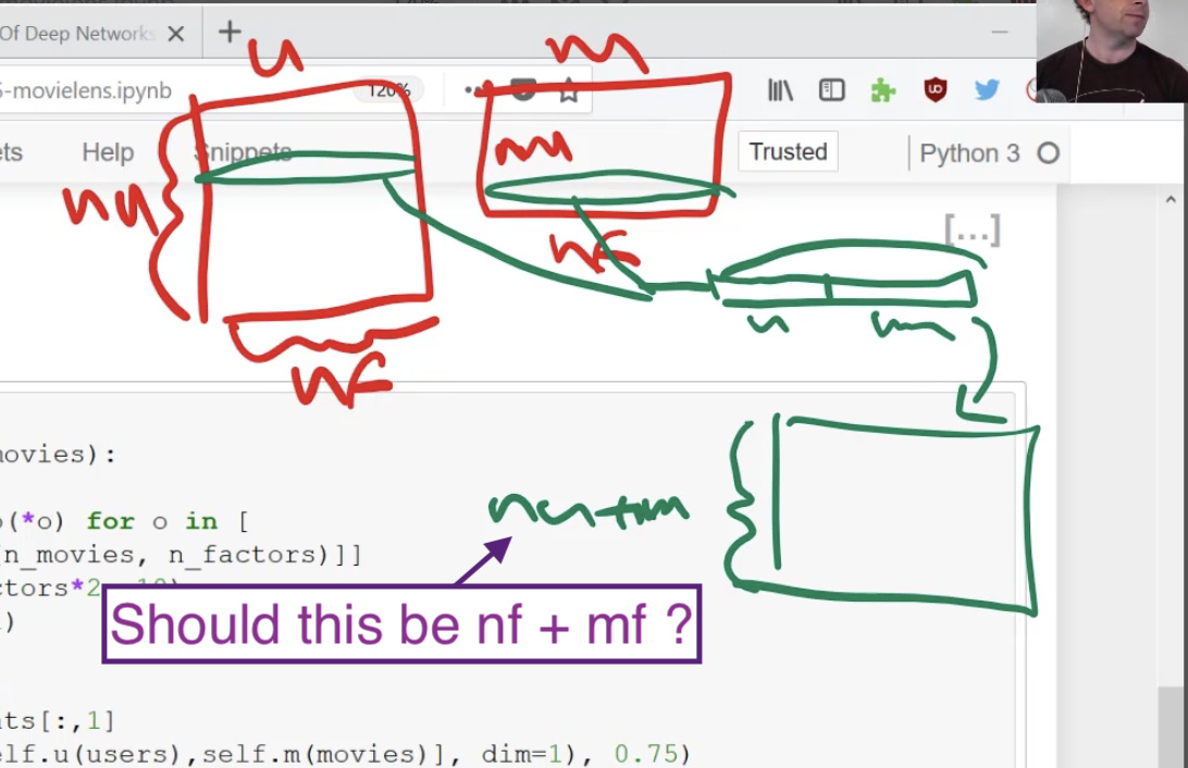
I’m a little confused when Jeremy says that we’re going to multiply our concatenation of user and movie lookups by a matrix that has nu + mu number of rows. My understanding is that it should be nf + mf instead, no? Because when we take extracts from U and M each has a length of nf and mf accordingly and after concatenating them we get nf + mf.


 "
"