I did watch again the video of the lesson 1 (part 1) to get the whole image and I took notes of the vocabulary used by @jeremy.
Let’s play ! OK ?
Can you give a definition / a url / an explanation for all the followings terms and expressions ?
If yes, you are done with the first lesson !!!
PS : you do not want to test yourself or you want to check your answers ? Go to the blog post “Deep Learning 2: Part 1 Lesson 1” of @hiromi : " super travail !!! "
course Fastai
forum Fastai
GPU
CUDA
NVIDIA
Crestle / PaperSpace
jupyter notebook
Data Science
SHIFT + ENTER in a jupyter notebook
python 3
wget
exclamation mark in a cell (ex : !ls)
bash command
python variable into brackets
training set
validation set
Fastai Machine Learning course : prerequesite or not ?
image Classifier
label
keras
plt.imread
plt.imshow
python 3.6 format string
img.shape
3 dimensional array (rank 3 tensor)
Red Green Blue (RGB) pixel values between 0 and 255
kaggal competition
pre-trained model
resnet24
ImageNet competition
Convolucional Neural Network (CNN)
accuracy
train a model
3 lines of code
epoch
testing set
learning rate
loss function
cross entropy loss
validation and testing set accuracy
Fastai library
transfer learning
pytorch
tensorflow
network architecture
data augmentation
validation set dependent variable val_y
data.classes
classes
object data
object learn
the model
prediction on validation set
learn.predict()
log of the predictions : log_preds
get the predictions on validation set np.argmax(log_preds, axis=1)
get probabilities on dogs : np.exp(log_preds[:,1])
numpy
top-down, the whole game
code driven approach
world class neural network
stalelite images
structured data
NLP classifier
recommendation system
text generator
create our own architecture from scratch
donwload a pre-trained model and precompute
alphago
image classifier for fraude dectection
machine learning
Arthur Samuels, 1950s, ML father
IBM mainframe
play checkers
traditional Machine Learning
features engineering
domaine experts and specialits
algorithm (Deep Learning) :
** infinitely flexible function
** all-purpose parameters fitting
** fast and scalable
neural network, number of simple linear layers interspersed with a number of non linear layers
universal approximation theorem
Fit parameters, Gradient Descent (how good are they, find a minimum on loss function curve, local miminim)
minimum time, GPU 10 time faster than a CPU
hidden layer
increase of number of parameters by layer is a problem but increase number of layers is teh solution
DL = neural network with multiple hidden layers
Google starts using DL in 2012
Geoffrey Hinton, DL father
Andrej Karpathy
inBox by Gmail
Skype Translator
Semantic Style Transfer
cancer detection
true/false positive/negative
CNN, Convolucional Neural Network
convolucional
find edges
multiplication of pixels values by a kernel (filter)
linear operation
linear layer
non linear layer
sigmoid
Relu
element wise multiplication
michael Neslon
Stochastic Gradient Descent
derivative
small step
learning rate
combine convolution, non linearity, gradient descent
picture of what each layer learns
parameters of the kernels are learnt using gradient descent
learn.fit()
learning rate not too high, but not too low as well
choosing a learning rate
learn.lr_find()
best improvement of the loss before it gets worse
learn.shed.plot_lr()
learn.sched.plot()
mini batches
traing loss
validation loss
validation accuracy
overfitting : stop fitting your model
tab to get list of function
SHIFT + TAB (once : parameters, twice : documentation, 3 times : pops up a window with source code)
Binary loss represents the loss function for a binary classification problem. This does not necessarily mean that the loss itself is normalized from 0 to 1.
y here represents the labels for the examples that the loss is calculated for. For example, if picture 1 is a dog and picture 2 is a cat, then y = [1, 0] (assuming 1 represents dog and 0 represents cat). p represents the probability that the example is a dog (1), output by the model.
I’m guessing that acts stands for actuals, as in the actual labels.
I’m not sure why you would want to get y from the confusion matrix. As I understand, the confusion matrix is a visualization of the model’s predictions so that you can see which categories your model performs well on and which ones it performs poorly on.
Setting precompute to True ensures that the model uses precomputed activations for the model. This means that the model will use the activations that were precomputed during training except for the last layer. This is because with little data, it will be difficult to properly train the whole model, but training only the last layer is easier to do.
At minute 49:27 in the video, I see a function S(x) = 1/(1-exp(x)). Is that an activation function? I seems to look like a Sigmoid, but that is 1/(1+exp(-x)).
Did a git pull and conda env update this evening and now lesson1.ipynb (for cell 29) gives AttributeError: 'ConvLearner' object has no attribute 'data_path'.
What is the relationship between epoch and batch size? How to set batch size correctly?
At 1:19 the teacher is talking about epoch and batch size, at each epoch we take a batch size of 64…
I noticed I was unable to plot the learning rate learn.sched.plot() until I set the batch size to 6 for my 200 images (100 each of each type) with a setting of 75% training 15% valid. When I inspected the current batch size learn.data.bs it was already set to 64 before I changed it for my dataset.
Hi prairieguy,
I get an error “selenium.common.exceptions.WebDriverException: Message: Process unexpectedly closed with status: 1” when i run the script. Could i be doing something wrong?
The issue with np.mean() and the call to accuracy_np(probs, y) failing as it was getting passed a one-dim array:
AxisError: axis 1 is out of bounds for array of dimension 1
update: for some reason pip wasn’t loading the latest version of fastai - I replaced it with pulling directly from github and it all works now. So it was a false alarm.
Ideally we would want to find a global minimum of our loss function which should represent “how far away” we are from our desired values. But in practice we may end up with overfitting.
From this paper: https://arxiv.org/abs/1412.0233
We empirically verify several hypotheses regarding
learning with large-size networks:
• For large-size networks, most local minima are equivalent and yield similar performance on a test set.
• The probability of finding a “bad” (high value) local minimum is non-zero for small-size networks and decreases quickly with network size.
• Struggling to find the global minimum on the training set (as opposed to one of the many good local ones) is not useful in practice and may lead to overfitting.
Hi just some feedback. I was following an older version of this course a while ago, and I found that much, much easier to follow than this version.
The old one had a few utility methods and stuff (“utils.py” and “vgg16.py”!), but this new one comes with thousands of lines of “helpful” code in the fastai library, way too much to casually understand without a lot of work.
Now I feel like I’m not learning how to use keras or theano or tensorflow or pytorch, I’m just investing a lot of time into learning your made-for-this-course framework.
I’m willing to work hard, but if I put in the work to understand the fastai library it’s not transferrable or useful. I’d much rather have to slowly build up over time all the code for image-loading, transforming, model creation, etc. Then at least that effort teaches me something that’s useful in the future.
As helpful as the fastai library is, it’s not likely to be used outside of this course. Rather than learn it, I’d like to learn how to do those things myself.
Can we please move the link to auto generate test data to a more prominent position in the wiki? I didn’t pay enough attention to this link until I actually spent considerable time to find web scrapers, download and arrange images into folders and be satisfied with my hours of work before realizing there was an easier way to do it.
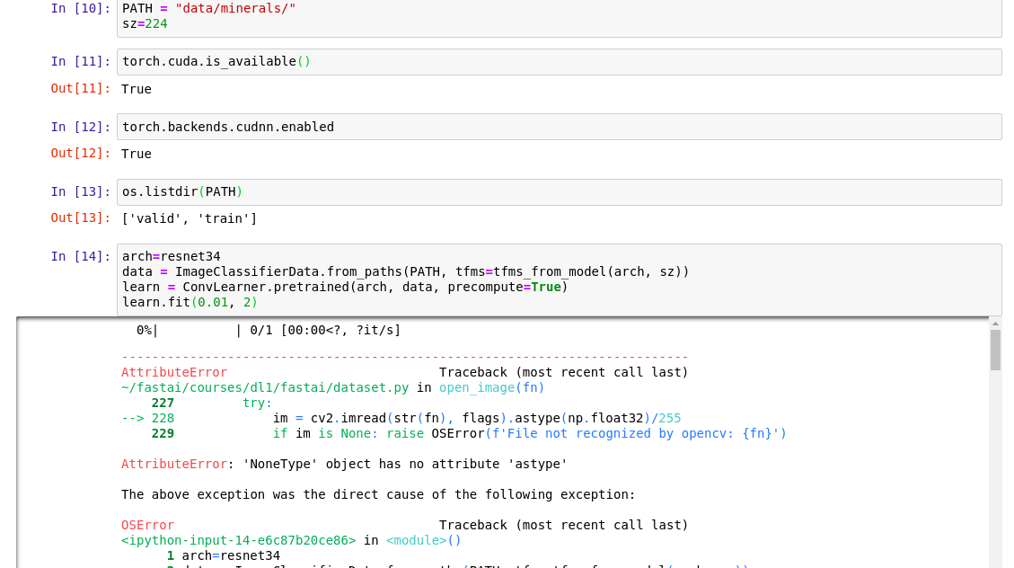
In lesson 1 around the 29th minute, @jeremy says that you could download some pictures, change the path to point to those pictures and use the same lines of code to train the neural network to recognize those images too.
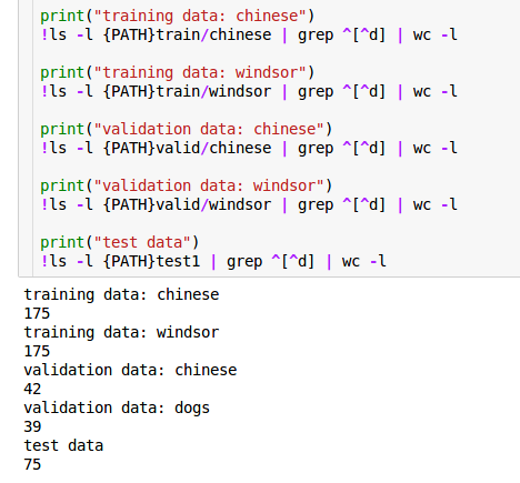
I wanted to train it to recognize minerals so I downloaded some pictures of 2 minerals and changed the path to point to the folder containing them but I’m getting some errors with the code.
I remember there was a link to a pdf where someone had made notes commenting in the Jupiter notebook itself and explaining the codes. Anyone know where I can find that?


 "
"