I didn’t know that Gabor filter initialization was implemented in Caffe. I’ve wondered about this since the paper “How transferable are features in deep neural networks?” says “on the first layer they learn features similar to Gabor filters”. I’ve also wondered about initializing the weights to discrete cosine transforms (DCT), suitably normalized like msra. Has anyone done experiments with either of these initializations? Is training any faster? And is the performance any better?
Update on Progressive Resizing Idea: (i.e Increasing the Image size as training progresses)
Workflow and Experiments:
- Plain Vannila Model with One Cycle Learning
- Plain Vannila Model with Cosine Annealing
- Progressive Image Resizing with One Cycle Learning
- Progressive Image Resizing with Adaptive Reduction in Batch size with One Cycle Learning
Took the CIFAR10 dataset and trained few epochs with size 32 and kept doubling it till 128
Batch size: 256 (Was not able to use 256 GPU memory issues). - For first two experiments
Learning Policy : One Cycle Learning
i.e learn.fit( lr, 1, cycle_len=15, use_clr_beta=(10, 13.68, 0.95, 0.85), wds=1e-4)
Here are my Observations:
epochs = 15
Progressive Resizing : szs = [32,64,128]
Batch Sizes : bss= [512,256,128]
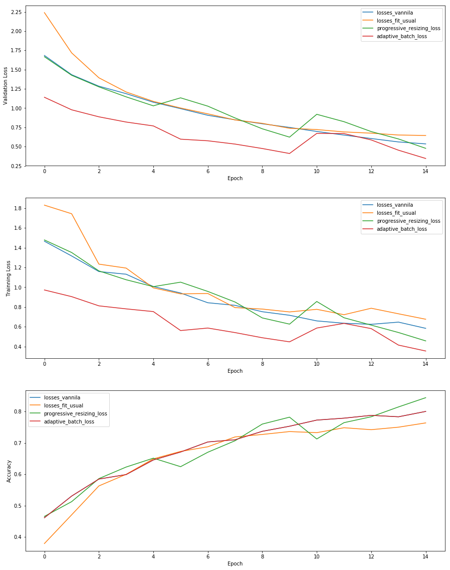
Bumps are due to Changes in Image Size/Batch Size. Varying the Image size and batch size seems to work the best among them.
When tried for longer epoch cycle there is no much gain in performance and the later methods become computationally expensive for a very meager improvement.
I have a feeling that if we elongate the number of cycles as the image resizing happens then we would be able to have better performance compared to all of them.
Experiment             Total Epochs  trn_loss	val_loss	accuracy
losses_vannila	             15   	 0.53523	0.583793	0.8001
losses_fit_usual	         15	     0.644244	0.675924	0.7635
progressive_resizing_loss	 15      0.477568	0.456707	0.8439
adaptive_batch_loss	         15      0.345881	0.35437	    0.8839
@jeremy @Leslie and others please share your thoughts !
P.S : Will update the associated notebook after i clean up the code
1 Like
Very interesting.
Questions:
- What architecture are you using?
- Why the inconsistency between the accuracy table and the plot? The plot shows the green curve as the highest final accuracy but the table says the combined image/batch resizing is best.
- What is the LR range? I am ignorant of the fastai implementation.
- What is the size of the validation data?
Another initial thought is that you are using Cifar and resizing it larger, which introduces blur. Better might be to resize imagenet down and test on the original, pristine validation images.
I am somewhat surprised by the magnitude of the improvement from the resizing and would like to sort it out in my mind.
Hi,
I have been playing about using the training phases note book and increasing the number of images in training using the one cycle provided in the notebook and using the darknet architecture on a GTX 970. I created CSV files with the different number of images (10, 100, 1000). I have a link to my notebook
As @urmas.pitsi pointed out I need to reset my model so my results don’t show anything of worth at the moment. but could be useful for people wanting a quick and dirty starting point!
2 Likes
nice!
-
if you want to reset and start from scratch then run this cell again:
m = Darknet([1, 2, 4, 6, 3], num_classes=10, nf=32)
otherwise your training will just accumulate on the same model. -
seems that your training and validation data is overlapping, that is why we see validation_accuracy=1.0
when you create phases, it could be that one phase trains on the data that will be in validation set for another phase. I may be wrong here, but it seems so at a glance:
df2 = pd.read_csv(PATH/‘train_10.csv’)
val_idx2 = get_cv_idxs(len(df2))
df3 = pd.read_csv(PATH/‘train_100.csv’)
val_idx3 = get_cv_idxs(len(df3))
df4 = pd.read_csv(PATH/‘train_1000.csv’)
val_idx4 = get_cv_idxs(len(df4))
df5 = pd.read_csv(PATH/‘train_2000.csv’)
val_idx5 = get_cv_idxs(len(df5))
df6 = pd.read_csv(PATH/‘train_3000.csv’)
val_idx6 = get_cv_idxs(len(df6))
Cheers! I thought something was a bit wrong with it! I will change my code later. and re test it!
I’ve read the wide resnet paper upon your question. I am actually not sure why activation is multiplied by 0.2 before addition in BasicBlock (which is a full pre-activation res block). That might be a good number that worked well in this case, I’m not sure  Maybe we can wait for dawn bench team to reply, I am also curious.
As I’ve played around for quite extensively with this wideresnet, it seems that 0.2 is pretty good choice  I tried without it and various other constants, but none have the performance of 0.2.
2 Likes
So it acts as a weighted sum, I wonder what happens if we make it a learnable parameter for general resnet s 
1 Like
@Leslie
Partial sampling in training for ImageNet amongst other cool stuff.
https://arxiv.org/abs/1805.08249
Thanks to @jeremy for tweeting that. Are they also using kind of similar idea to Jeremy’s: making disjoint class groups?
Could you write me short sample how it could be done in pytorch, just line or 2 of code? I could test it right away
I am still learning the pytorch way of deep learning…
I am not sure but this might maybe work, haven’t test it:
Idea is we will define weight as a learnable variable by setting requires_grad=True during initialization. Then autograd optimizer should do the rest as it will be added to computational graph I suppose.
class BasicBlock(nn.Module):
    def __init__(self, ni, nf, stride, drop_p=0.0):
        super().__init__()
        self.bn = nn.BatchNorm2d(ni)
        self.conv1 = conv_2d(ni, nf, 3, stride)
        self.conv2 = bn_relu_conv(nf, nf, 3, 1)
        self.drop = nn.Dropout(drop_p, inplace=True) if drop_p else None
        self.shortcut = conv_2d(ni, nf, 1, stride) if ni != nf else noop
        self.weight = Variable(torch.FloatTensor(1,).uniform_(0, 1), requires_grad=True)

    def forward(self, x):
        x2 = F.relu(self.bn(x), inplace=True)
        r = self.shortcut(x2)
        x = self.conv1(x2)
        if self.drop: x = self.drop(x)
        if (self.weight.data[0] < 0) | (self.weight.data[0] > 1):
            self.weight.data = torch.clamp(self.weight.data, 0, 1)
        x = self.conv2(x) * self.weight #0.2
        return x.add_(r)
2 Likes
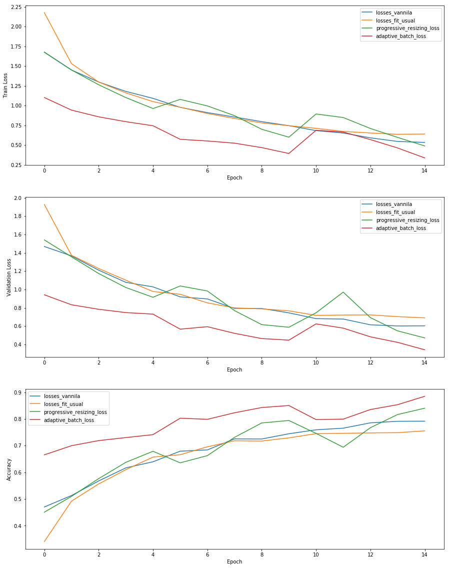
- I am using the Same architecture @deanmark used. (i.e Resnet2([16, 32, 64, 128, 256], 10, 0.2) )
- Sorry Found a bug when plotting the results. Here is the updated version of plots:
- LR : i had used LR varying from 1e-2 to 1e-3 i guess
- I am using the entire test set as validation set.
Notebook is made available : Link
Thats True! Fastai DAWN Benchmark uses Progressive Resizing i believe. I am not sure how well it had contributed to the whole of training process. Will try to setup the same experiments with Imagenet and check it out.
P.S : I find the training times to increase with the resizing approach. It almost takes 12 minutes on p2.xlarge (AWS) for the normal Training procedure and Takes almost 3x i.e 35-36 minutes for the resizing approaches ?
What could be the reason for the increase in time ?
- Bottleneck between CPU and GPU ?
- Under Utilization of GPU in Earlier Stages due to small batch size. if thats the case then adaptive batch should train faster (Actually it does but it is very negligible. Say 2-3 mins faster)
~Gokkul
- I don’t understand what
represents. It is a resnet but with how many layers?
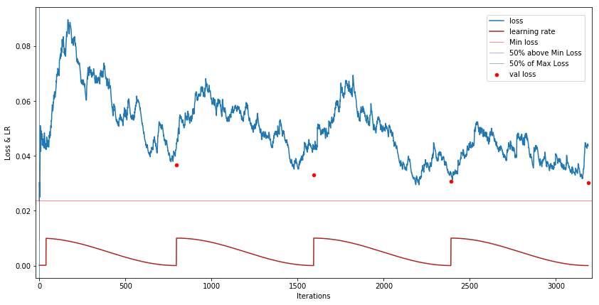
3. I’m surprised by the low learning rates but it does explain why I’m not seeing the characteristic 1cycle shape. For resnset and 1cycle, I’d expect LR to go from 0.1 to 3 down to 1e-3. Also, I’d expect a final accuracy near 90% for the baseline, not 80%.
I believe the increase in training time is because you are resizing larger, not smaller. I understand progressive resizing as a coarse to fine approach - start with a quick training with a coarse set of training images, transfer the weights, then train with the original images.
There’s no point increasing size to be larger than the original image. In this case, cifar10 is 32px images, so that’s the largest you should go. (Also, cifar10 are too small to be usefully down-sized, so as @Leslie said, you should try this on imagenet or similar instead.)
4 Likes
Just w2v, like we did in the DeVISE lesson.
2 Likes
Hi everyone. I made a baseline notebook using MNIST. To Leslie and Jeremy: this doesn’t contain any relevant experiments. But it has served as a good warm up.
I expect to have a notebook of experiments on CIFAR-10 out, if not by Monday, then by the end of the week – and ImageNet later if things look good (or for work on larger images).
Navigation help for anyone looking at the notebook:
- Data setup
- Architecture setup
- Loss Function
- Training (with plots)
- Testing
- More training & testing (with plots)
- Closing notes (with table of results)
A couple pictures:
-
A pretrained ResNet18 training only the classifier head (1st epoch):
-
A custom CNN in its last 4 of 7 training epochs:

Aside from the research, this has taught me alot about pytorch and fastai’s internals. Apparently there’s a built-in callback to save the best version of a model which I look forward to testing out.
3 Likes
Hi Dean,
Can you please share your thoughts around this notebook, I planned this to account for all the possibilities in the approaches shared by Leslie and Jeremy. I will plug it into the notebook shared by Radek to test DAWNBench.
I also have few questions around the updated approach you had shared but I’ll PM you those questions. Eagerly awaiting your reply.
Thanks
Hi @PranY,
Dynamic resizing is already built into the fastai library, so better just use that. Look at the “dl1/lesson2-image_models.ipynb” notebook for an example. On top of that you can use my code to select which classes to use. I would use this code to change the data object on the fly:
cls_list = [0,4,3,5]
learn.set_data(get_data(sz, cls_list))
def get_data(sz, classes):
    tfms = tfms_from_model(f_model, sz, aug_tfms=transforms_top_down, max_zoom=1.05)
    return ImageClassifierData.from_csv(PATH, 'train-jpg', label_csv, tfms=tfms,
                    suffix='.jpg', val_idxs=val_idxs, test_name='test-jpg', partial_train_classes=classes)
The partial_train_classes argument is enabled with my code. You also have a max_train_per_class argument to restrict the number of training images per class as per Leslie’s idea. Every time you finish several epochs, you can change the data object to use different sizes and different classes. This approach allows you to use any previous fastai code with minimal change.
5 Likes