A stride of 3 would reduce the grid by 3x, not 2x. Try working through the convolution arithmetic tutorial to make sure you understand the formula that @wdhorton mentioned above http://deeplearning.net/software/theano/tutorial/conv_arithmetic.html
For small inputs the formulas break down For feature maps with even dimensions and a (3, 3) kernel with a stride of 2 the dimensions don’t get halved. (We could pad the input on one side only but not sure if that is an okay thing to do?)
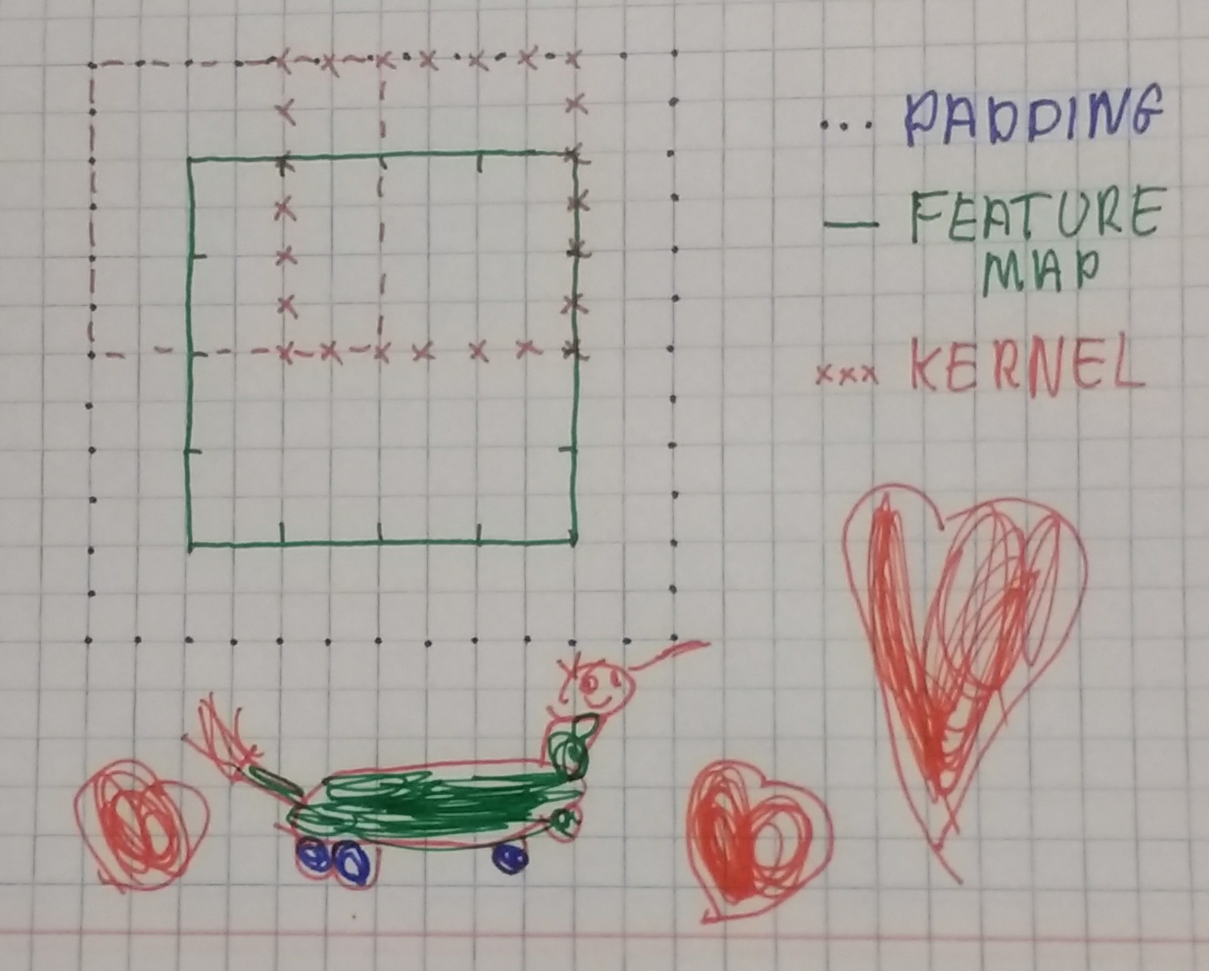
Apologies for the additional drawings but had a little bit of fun with my 5-yr old and I think she is very proud to see her work published on the forums  For a
For a (4, 4) feature map I think pad=1, kernel=3, stride=3 would give us a (2, 2) output that we get here but doubt those were the settings that were used as we would be looking at a lot of zeros vs the feature map content.
So the question still remains open How did we go from (4, 4) feature map to (2, 2) Guessing we went for a ‘(2, 2)’ kernel with a stride of 2, but what did we do then for going from (7, 7) to (4, 4) and why the difference?
Might be I am reading into this too much and I know I can get the numbers from the notebook. I wonder though if there is a reason behind the params that we used (and I don’t see how both convolutions can share same params) that goes beyond producing the shape that we want.
EDIT: I kept thinking and realized this has nothing to do with the feature map size (as it will work for a (3x3) feature but everything to do with the even / odd dimension sizes. I guess this must mean that using one side padding is a common practice?
11 Likes
The most challenging part in this lesson for me was the whole process of writing the loss function. As I was trying to redo it from scratch, I found myself constantly peeking at Jeremy’s notebook to check if my intermediate results were consistent with what he found, which lead to a lot of cheating.
So to see if I really could do it, I saved all those intermediate results closed the notebook and waited the next day before I reopened a blank notebook and tried again. After lots of frustrations and debugging here is the result, the notebook with the associated numpy arrays saved. Hope it can help anyone who is struggling!
In the end, I still cheated once, and I still don’t really get the use of .cpu() and .continuous() in
def one_hot(labels):
    lbls = torch.eye(nb_classes+1)[labels.data.cpu()]
    return V(lbls[:,:-1].contiguous())
5 Likes
I just put them in there because pytorch complained if I didn’t  (if you try to use a function that requires a contiguous tensor, and yours isn’t, it’ll tell you directly).
2 Likes
Oh, pytorch did complain!  The error message for the contiguous was clear, that’s true. It’s the .cpu() I really wouldn’t have found without going back to the notebook.
Not sure if it is helpful to anyone but I got: Input type (CUDAFloatTensor) and weight type (CPUFloatTensor) should be the same, while running pascal_multi notebook:
batch = learn.model(x)
replacing .cpu() with .cuda() fixed it for me:
for i,o in enumerate(y): y[i] = o.cuda()
learn.model.cuda()
anchors = anchors.cuda(); grid_sizes = grid_sizes.cuda(); anchor_cnr = anchor_cnr.cuda()
8 Likes
I was introspecting the shapes of the dataloader batch after the following code:
trn_ds2 = ConcatLblDataset(md.trn_ds, trn_mcs)
val_ds2 = ConcatLblDataset(md.val_ds, val_mcs)
md.trn_dl.dataset = trn_ds2
md.val_dl.dataset = val_ds2
x,y=to_np(next(iter(md.val_dl)))
x.shape,y[0].shape,y[1].shape gives
((64, 3, 224, 224), (64, 56), (64, 14))
I am not able to understand why the y[0] and y[1] shapes are 56 and 14.
Does anyone why the shapes are like that.
from my understanding y[0] should refer to bounding boxes, and y[1] to classes. But the shapes don’t make sense.
1 Like
Hi Phani,
Different minibatches have differently sized y[0] and y[1] shapes depending on how many ground-truth objects are in the the images within that minibatch.
For a given batch, I think the y shape is determined by the image therein with the most objects in it - so, for the mb you grabbed, the 14 for y[1] means the image with the most objects has 14 objects**, and in turn, y[0].shape is 4 bbox coords * max # of objects in the batch = 4 * 14 = 56.
If you call the following code, you can see a list that corresponds to the y[1] shape (i.e., the max # of objects, if I am interpreting it correctly) in each of the 8 mini-batches in the validation set.
val_mb = list(iter(md.val_dl))
[i[0] for i in (o[1][1][1].shape for i,o in enumerate(val_mb))]
It returns:
[14, 7, 9, 16, 9, 17, 11, 11]
This means that our loss function has to flexibly adjust to the shape of our target, though the number of predictions we make is always constant, no matter the ground truth of the images: # of anchor box archetypes per grid cell (k) * # of grid cells * 4 * (num_classes + background).
**(Hi! Edited for clarity: y[1] isn’t the max # of classes, but rather the max # of total objects - i.e., many images have several objects of the same class, like the one with several ‘person’ instances in the lesson notebook)
18 Likes
thanks @choews for the great explanation.
1 Like
This error stumped me for a while too. At least I learned a lot about sending things to and fro.
As I think more about this approach, this flexibility of dealing with varying tensor sizes across mini-batches seems to be one of the upsides of frameworks like PyTorch which use dynamic computation graphs in comparison to frameworks like TensorFlow etc. Can we achieve similar elegance with TF? Spare my ignorance.
1 Like
Seems that whether we use one side padded convolutions at some point and what their exact parameters are is relatively unimportant vs the big picture.
Forget the architecture, it’s just a thing that is spitting out 16 x (4 + c) activations (~ 1h:20m)
Seems the magic lives in the cost function and despite the arch being fancy it is still ‘just’ a universal function approximator
I think I was blowing the importance of a minor detail way out of proportion then.
Thank for @daveluo to unpack the SSD_MultiHead and reconcile the output shape.

Edit: See corrections and more detail explanation below:
9 Likes
Seriously, great job, helped a ton! 
Getting good understanding of each layer, especially in places of intersection between two models (in this case how convolution proceeds after base model renet34 to calculating the final layers to match output activations), how they are put together is very important. Actually I think this gives us an opportunity to get into the head of these model developers.
You are doing a good job by being curious, and helping us around.
Thanks for the photo share! It was really helpful and great learning for me too to work it through with you all.
A correction to make at the bottom-left of the photo where it says “Output = (64, 189, 4)”:
- 64 is the batch size, not channels
- 189 is the number of predictions for each of the 64 images in the batch. This represents/corresponds to the 189 anchor boxes that we defined up top.
- 4 is the set of bounding box corners that is trained to define each anchor box (x 189 from the 2nd dimension). This is the 1st of 2 outputs in a list (specifically,
torch.cat([o1l,o2l,o3l], dim=1)])
The second output has 21 elements in the 3rd dimension - full shape would be (64,189, 21) - representing the one-hot encoded predictions for the 20 categories + 1 ‘bg’ category. This is torch.cat([o1c,o2c,o3c], dim=1)
from the return step of the forward pass:
class SSD_MultiHead(nn.Module):
    def __init__(self, k, bias):
        super().__init__()
        self.drop = nn.Dropout(drop)
        self.sconv1 = StdConv(512,256, drop=drop)
        self.sconv2 = StdConv(256,256, drop=drop)
        self.sconv3 = StdConv(256,256, drop=drop)
        self.out0 = OutConv(k, 256, bias)
        self.out1 = OutConv(k, 256, bias)
        self.out2 = OutConv(k, 256, bias)
        self.out3 = OutConv(k, 256, bias)

    def forward(self, x):
        x = self.drop(F.relu(x))
        x = self.sconv1(x)
        o1c,o1l = self.out1(x)
        x = self.sconv2(x)
        o2c,o2l = self.out2(x)
        x = self.sconv3(x)
        o3c,o3l = self.out3(x)
        return [torch.cat([o1c,o2c,o3c], dim=1),
                torch.cat([o1l,o2l,o3l], dim=1)]
7 Likes
Going back to the initialization of the bias on the output convolutional layer that gives us the predictions of classes (-3 when we have 16 anchors, then -4 when we have a lot of anchors), Jeremy has stated that he put a negative value to make it harder for our the network to predict a category (to make it easier to predict background, which happens a lot of time).
I’ve played around with this in that notebook and I’ve come to several conclusions.
-
It’s super helpful to do this indeed, because even with a lot of training, a network where we initialize the bias with zeros doesn’t train as well, and doesn’t manage to come to the same results in terms of loss.
-
Contrary to what I thought at first, the network won’t learn on his own to put a strong negative value in those bias. In fact, they barely change during the training.
-
The best value for initialization (in the sense that it gives the lower validation loss after a cycle) I found by trying a lot of them is -6 for the first model with only 16 anchors.
Then I tried to find a way to guess what the ideal value would be for this initialization without trying a lot of them and doing a cycle. My idea was to try all the bias in a given range on a model and test them on the first mini-batch, then compute the loss. Then I’d initialize the bias to the value that gave the minimum loss.
In the first model with 16 anchors, this gave me -5.45, not as good as the empirical -6, but close enough.
On the last model with all the anchors and the focal loss, it gave me -3 (close to the -4 Jeremy picked) which then gave similar results after a lot of training (final validation losses of 5.523 and 5.497 respectively).
9 Likes
I got this error to. The line
anchors = anchors.cpu(); grid_sizes = grid_sizes.cpu(); anchor_cnr = anchor_cnr.cpu()
happens after the error about weight type and input type.
I found .cpu() in a number of places:
def one_hot_embedding(labels, num_classes):
    return torch.eye(num_classes)[labels.data.cuda()]

for i,o in enumerate(y): y[i] = o.cpu()
learn.model.cpu()
I changed it and now do not get the runtime error about CUDAFloatTensor vs. CPUFloatTensor.
Now I get the error
Performing basic indexing on a tensor and encountered an error indexing dim 0
with an object of type torch.cuda.LongTensor. The only supported types are integers,
slices, numpy scalars, or if indexing with a torch.LongTensor or torch.
ByteTensor only a single Tensor may be passed.
I did a little looking into it, but I have to go right now. More later.