Lesson 2 discussion

Hi Jeremy,

I am trying to do the state-farm-distracted-driver-detection as you suggested from scratch and I get stuck in the very beginning when I try to create my validation set.
In dogs and cats redux you do:
g = glob(’*.jpg’)
shuf = np.random.permutation(g)
for i in range(50): copyfile(shuf[i], DATA_HOME_DIR+’/sample/valid/’ + shuf[i])

But this does not work out for the sate farm competition. Could you help me figuring out how to create such sets

Do we need to do a sample set as well ?

Thank you so much

I’m trying to understand the keras code in vgg16.py. Can someone point me to where in the keras documentation it explains what members a image.ImageDataGenerator() would have i.e. nb_sample etc? I couldn’t find it on the doc page: https://keras.io/preprocessing/image/

For any Python newbies (like me) who were baffled by the following line in the lesson 2 notebook…

np.array(OneHotEncoder().fit_transform(x.reshape(-1,1)).todense())

Passed into this was something like val_batches.classes which is an array with 2000 elements, where each element is a 0 or 1 depending on whether it’s a dog or a cat. In this example i’ll use a simplified example.

classes = np.array([0, 1, 0])
# array([0, 1, 0])
classes.reshape(-1,1)
# array([[0], [1], [0]])
OneHotEncoder().fit_transform(classes.reshape(-1,1))
# <3x2 sparse matrix of type '<type 'numpy.float64'>'
# with 3 stored elements in Compressed Sparse Row format>
OneHotEncoder().fit_transform(classes.reshape(-1,1)).todense()
# matrix([[ 1., 0.], [0., 1.], [1., 0.]])
np.array(OneHotEncoder().fit_transform(classes.reshape(-1,1)).todense())
# array([[ 1., 0.], [0., 1.], [1., 0.]])

Notice that in our initial array the first value is 0 and in the final output this is encoded as [1., 0.], which would make sense if you imagine how the fit_transform() function maps new unique values as it encounters them.

As Rachel and others point out, keras.utils.np_utils.to_categorical(classes) yields the same result. I cannot see in the Keras documentation how anyone would know about the np_utils namespace though.

1 Like

I am trying to understand the effect of batch sizes on a simple linear model example from lesson 2. The notes say larger the batch size which intuitively makes sense. Specifically, this is the line I have a question about:
With a batch_size of 1 I get the following results:
lm.evaluate(x,y, verbose=1)
10.702649688720703
lm.fit(x, y, batch_size=1, nb_epoch=10, verbose=1)
Epoch 1/10
50/50 [==============================] - 0s - loss: 0.6443
Epoch 2/10
50/50 [==============================] - 0s - loss: 0.0438
Epoch 3/10
50/50 [==============================] - 0s - loss: 0.0143
Epoch 4/10
50/50 [==============================] - 0s - loss: 0.0060
Epoch 5/10
50/50 [==============================] - 0s - loss: 0.0023
Epoch 6/10
50/50 [==============================] - 0s - loss: 8.8335e-04
Epoch 7/10
50/50 [==============================] - 0s - loss: 3.3827e-04
Epoch 8/10
50/50 [==============================] - 0s - loss: 1.4953e-04
Epoch 9/10
50/50 [==============================] - 0s - loss: 5.8482e-05
Epoch 10/10
50/50 [==============================] - 0s - loss: 2.3806e-05

And you see that it converges reasonable quickly. However when I increase the batch size to 10, my understanding is that it should take 10 pairs of y = 2x1+ 3x2+1 and run the stochastic gradient. However I see that the convergence is actually much slower which seems counter intutive:
lm.evaluate(x,y, verbose=1)
9.9358782577514653
lm.fit(x, y, batch_size=10, nb_epoch=10, verbose=1)
Epoch 1/10
50/50 [==============================] - 0s - loss: 4.0266
Epoch 2/10
50/50 [==============================] - 0s - loss: 0.4919
Epoch 3/10
50/50 [==============================] - 0s - loss: 0.3260
Epoch 4/10
50/50 [==============================] - 0s - loss: 0.2758
Epoch 5/10
50/50 [==============================] - 0s - loss: 0.2356
Epoch 6/10
50/50 [==============================] - 0s - loss: 0.2013
Epoch 7/10
50/50 [==============================] - 0s - loss: 0.1718
Epoch 8/10
50/50 [==============================] - 0s - loss: 0.1481
Epoch 9/10
50/50 [==============================] - 0s - loss: 0.1256
Epoch 10/10
50/50 [==============================] - 0s - loss: 0.1052

What am I missing here?

Difference between getting images using imagedatagenerator with class_mode=None vs class_mode=‘categorical’. I dont see a separate one hot encoded label field in the acquired directoryiterator. The only difference is when i try to concatenate batches.next similar to get_data it returns an error about shape in data acquired using class_mode categorical and accepts None but when i check image_shape both the data has same shape(3,224,224).

Hey,

I’m trying to replicate the optimization function presented in the video from Lesson 2. However, I can’t replicate the results shown with the same Learning Rate as in the video.

Here’s my code:

def optimizeGD(initial_a, initial_b, xs, ys, iterations, lr):
    curr_a = initial_a
    curr_b = initial_b
    curr_error = loss(curr_a, curr_b, xs, ys)
    errors = np.array([curr_error])

    for i in range(0, iterations):
        # partial derivative of the loss function
        # d((y - (a*x + b))**2)/da = 2*x*(a*x + b - y) = x * (d(..)/db)
        # d((y - (a*x + b))**2)/db = 2*(a*x + b - y)
        
        dldb = 2 * (line(curr_a, curr_b, xs) - ys)
        dlda = xs * dldb
        
        # print np.mean(dlda) * lr, np.mean(dldb) * lr
        
        curr_a -= np.mean(dlda) * lr
        curr_b -= np.mean(dldb) * lr * 100
    
        curr_error = loss(curr_a, curr_b, xs, ys)
    
        errors = np.append(errors, [curr_error])
    
    return (curr_a, curr_b, curr_error, errors)

As you can see, I have to “boost” the learning rate for the “b” dimension. And, the learning rate I have to set to “0.0001” as opposed to “0.01” in the video. If I enter a LR greater than “0.0001”, my optimization function will not work; its loss will just get bigger and bigger.

Can someone point to a material where I can read about this type of issue? How can I improve my code? Am I expected to use different LR for each dimension?

Thank you :slight_smile:

I think I managed to get some progress on this!

The issue is in these lines:

dldb = 2 * (line(curr_a, curr_b, xs) - ys)
dlda = xs * dldb

In these partial derivatives, we are mixing dimensions, and the scale and magnitude of our X’s and Y’s will impact on our optimization function.

I’m not sure if it’s cheating or not, but I managed to solve this issue by making sure my points in either dimensions are in the same scale. I can always scale back the results to the actual values at the end.

Hello!
I’m trying to implement the code from lesson 2 using get_batches instead of get_data, as the later resulted in running out of memory, however I’m having some trouble generating the predictions for the test data.

So far I’ve managed to finetune the model by first popping the last layer of the vgg model and then adding a dense layer with only 2 outputs, followed by a fit_model (with 0.9785 accuracy).
For my validation set, I’'m trying to predict using
preds = model.predict_generator(val_batches, val_batches.nb_sample)
which outputs
array([[ 1., 0.],
[ 0., 1.],
[ 0., 1.],
…,
[ 1., 0.],
[ 0., 1.],
[ 0., 1.]], dtype=float32)

and then I try to plot the confusion matrix using
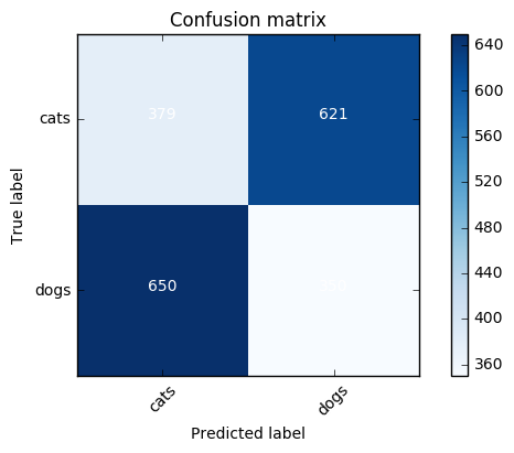
cm = confusion_matrix(val_classes, np.round(preds[:,1]))
plot_confusion_matrix(cm, {‘cat’:0, ‘dog’:1})

and I get these awful results:

So am I implementing wrongly lesson 2 using batches?
Thanks in advance!

Hi,

I might be a little late to the party on this, but I was having the same issue as a couple of the previous posters, in that I’m using my own PC, (Intel i5-7600K, 16Gb RAM, GTX 1070), and found that the get_data() function caused my RAM and Swap to rapidly fill up. It seems that the get_data() function’s overall output is just an array of features. So, instead of loading the entire image library into memory and predicting the entire batch, why not just load individual images, process the prediction for each image, and construct that final required prediciton array piece by piece?

To that end, I wrote a function which attempts to do this, then, matching the original Lesson 2 notebook, saves the final feature array to disk.

Please note, that although I’m by no means new to programming (25+ years), this (fantastic) course is the first time I’ve ever programmed using Python, so it’s quite possible that the following code is perhaps not as efficient as it could be, seeing that I’m not yet familiar with Python’s intricacies. It’s also possible (I hope not) that the final array is not “ordered” correctly (if that matters?)

Anyway, here’s the function and how to use it. Please feel free to take/improve as necessary. It also implements the Keras image library, so ensure that it’s imported too:

from keras.preprocessing import image

def get_features(dirname):
    #print(dirname)
    directory = os.fsencode(dirname)
    trn_features = []
    for dir in os.listdir(directory):
        subdir = os.fsencode(dirname + "/" + os.fsdecode(dir))
        for file in os.listdir(subdir):
            imgname = os.fsdecode(file)
            imgfile = os.fsdecode(subdir) + '/' + imgname
            #print(imgfile)
            test_image = image.load_img(imgfile,target_size=(224,224))
            test_image = image.img_to_array(test_image)
            test_image = np.expand_dims(test_image,axis = 0)
            result = model.predict(test_image,batch_size=1)
            trn_features.append(result[0])
    return np.array(trn_features)

To call it, simply pass the directory path. Use it as a drop in replacement for get_data()

trn_features = get_features(path+'train')
val_features = get_features(path+'valid')

It takes a while to process all 23,000 images, but it should (eventually) return an array with the same shape as trn_features in the original Lesson2 notebook:

trn_features.shape
(23000, 1000)

The, the array can be saved/loaded as required:

save_array(model_path+'train_lastlayer_features.bc', trn_features)
save_array(model_path+'valid_lastlayer_features.bc', val_features)

trn_features = load_array(model_path+'train_lastlayer_features.bc')
val_features = load_array(model_path+'valid_lastlayer_features.bc')

I hope that helps somebody!

Cheers,

Codegnosis.

Hi Stephani, (how) did you manage to get this error resolved? Could you please respond? thank you

Mak,

I am not sure what the error is I got resolved. Can you please cut n paste it in your reply as I can’t see what it refers to.

Cheers,

Stephen

I’m training the cats and dogs on a google cloud machine having Tesla K80 11GB GPU installed. It takes a longtime to train. I was wondering has anyone run the notebook on the whole dataset (23000) and if so, on which GPU and how long has it took to train a single epoch.

Thanks

Hey guys,

I’m following Jeremy’s solution for submitting the solution. Everything is fine up to the point where I run the fit

vgg.fit(batches, val_batches, nb_epoch=1)

When I run this line I get the following exception:
Exception: The model needs to be compiled before being used.

Has anyone seen this before?

1 Like

could anyone tell me what is the usage of vgg_mean in vgg16bn source?

It is used for input normalization. Input normalization is a common practice in machine learning. Typically you get inputs, subtract mean value and divide by standard deviation. See this Wikipedia article for details. Motivation: if you don’t do it, some of your inputs can be very large, and it leads to very large values of activation functions, your gradients will be large and it makes the model harder to train.
In our case we don’t need to divide by standard deviation because our inputs are in a constrained interval from 0 to 255, so we can just subtract mean values. vgg_mean is an array of mean values for every channel of ImageNet dataset.
Jeremy explains it in more details in Lesson 3.

Hey, so I kept trying to implement the code for this lesson by myself and the results are still disastrous.
Here is the relevant code

vgg = Vgg16()
model = vgg.model

model.pop()
for layer in model.layers: layer.trainable=False
model.add(Dense(2, activation='softmax'))

img_width, img_height = 224, 224
gen=image.ImageDataGenerator()
batches = gen.flow_from_directory(path+'train', target_size=(img_width, img_height), batch_size=batch_size, shuffle=True)
val_batches = gen.flow_from_directory(path+'valid', target_size=(img_width, img_height), batch_size=batch_size, shuffle=False)

opt = RMSprop(lr=0.1)
model.compile(optimizer=opt, loss='categorical_crossentropy', metrics=['accuracy'])

fit_model(model, batches, val_batches, nb_epoch=2)
which outputs val_loss: 0.3922 - val_acc: 0.97
probs = model.predict_generator(val_batches, val_batches.nb_sample)

However I keep getting

The reason for me to try and run the code using flow_from_directory and predict_generator is because running the code with the get_data function provided results in a “Cannot allocate memory” error. However these two functions give me bad results. I have read the documentation for these functions and cannot find what I am doing wrong. I’d be glad if someone could shed some light on this. Thanks in advance!

Francisco

Hi all,

I have a quick question regarding the differences between using Theano and Tensorflow backend, which may or may not be answerable!

So, I’ve run the exact same model using both backends, but the end results are quite different, with the 97.7% accuracy using Theano, but only around 91% - 92% using Tensorflow. I’m using the latest packages available for both backends, and was just wondering if there was a (relatively) simple answer as to why there is such a difference in results, when training the same model using the same data?

Cheers,

Paul.

3 Likes

One possible explanation was provided in Lesson 1 forum thread.
Theano and TensorFlow implement convolutional layers in different ways, and if weights for a Theano model are loaded into TensorFlow model, weights shall be converted.
I didn’t check if this conversion helps to get to 97-98% accuracy on TensorFlow. Please tell us about results if you try it.

1 Like

Hi,

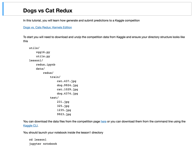
This might be a straightforward question to most with a stronger coding background, but I was wondering how Jeremy determined the folder structure that he needed to run his dog-cat redux code (see screenshot below)? I understand that this is the structure needed to run vgg16() but would be great if someone could point me to information on why the information needs to be structured this way. Thanks!

Hey @Codegnosis

I was looking to get a PC of similar specs to utilize instead of AWS and had a few questions if you didn’t mind :slight_smile:

How does it fair comparatively, or would you have any advice regarding setting it up out of the box?

What is your setup/ environment with this PC?

Thanks in advance,

Ian