Dropout amount in the classifier

[radek]

I suspect that fastai again provides us with very sensible defaults hence I could probably answer my own question by just looking at the library, but wanted to ask - what are some usual amounts of dropout people use in the fully connected part of a CNN that work well?

If I were to go by fastai defaults, I believe it would be 0.25 between the activation layer and the layer before softmax, and 0.5 between last layer and softmax.

The reason I am asking is that those amounts intuitively seem quite high - dropping half of the layer just before softmax sounds quite extreme!

I can see how the answer likely could be along the lines that this seems to have work best across a vast spectrum of applications and in general additional experimentation could be of value. Also, this likely is very dataset specific. (Need to reduce bias -> remove dropout, reduce variance -> add dropout).

Maybe there is no quick and easy answer apart from the defaults being a good starting point and there not being really much information on this subject, but if there would be any reading on this subject or any info that one might share that would be greatly appreciated (as in, some successful models, etc).

PS. As I was finishing this post I thought of googling this - I entered the name of one of my favorite writers and the term dropout and this is what I got:

Deep Learning for NLP Best Practices

I think the paper by Srivastava et al. is probably a great source of insight - planning to read it throughly, but if anyone would have any other materials they found useful or could shed some light on this please do share

[jeremy (Jeremy Howard)]

I’d be interested to hear what you find. 0.5 in last layer seems pretty standard. Most people don’t add 2 FC layers, so there is no standard there.

For RNNs, AWD-LSTM is the best practice for regularization.

[helena (helena s)]

for the anecdotal evidence, i’ve been testing various dropout values, for 2 FC type (4096 w) type CNN - 0.2/0.4 - overfit, 0.5/0.7 underfit - 0.5/0.5 combo seems like the best fit…
(along with the heavy batchnorming)

[Moody (Sarada Lee)]

@radek The reason I am asking is that those amounts intuitively seem quite high - dropping half of the layer just before softmax sounds quite extreme!

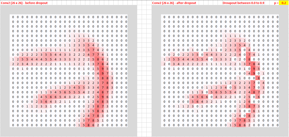
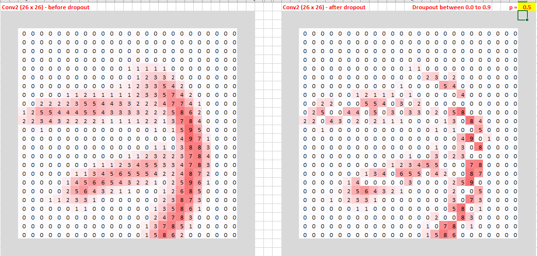
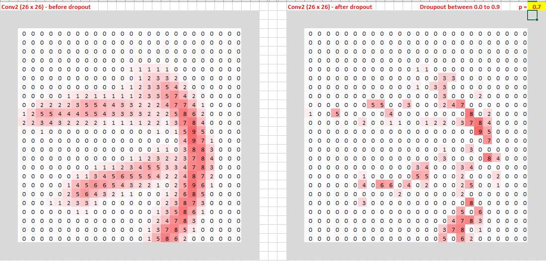
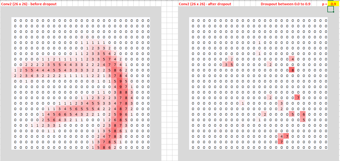
I also want to understand dropout ( p ) better by visualizing it. The following “No dropout” image is based on Jeremy’s conv-example.xlsx, Conv2 - 26 x 26 pixels.

No dropout vs p = 0.2

No dropout vs p = 0.5 (sounds high but we still can recongize number 7)

No dropout vs p = 0.7

No dropout vs p = 0.9 (very extreme!)

It is an interactive spreadsheet. Once the dropout rate is specified, it can randomize output every time. Ping me if you want to play with it.

[radek]

Quite an investigation you did there into this! Cool!

Thx for the spreadsheets. I have bypassed playing with them all together for the course and I also don’t have access to Excel

One thing I would like to mention. Here you are dropping out parts of the input itself. This generally would be referred to as adding noise I think (can be looked at as a technique of regularization). I think this is done only in very specific situations in research / real life applications (denoising autoencoder, experimenting with regularization via blanking out parts of input, blanking out parts of input to figure out which parts are important to our algorithm).

Generally, dropout would be added to later layers in the NN stack. If any is added to the convolution parts, those will be very small amounts. As it is added usually only in the fully connected layers, it is often quite hard to intuitively understand what it does with the features that the NN learns.

I like going to the basics and also for other reasons the original paper on dropout by Hinton is quite awesome.

Either way, apologies @Moody if this is not very useful that I share here.

The analysis you did is certainly interesting and useful! Thank you for sharing the images.

[Dee (Sean)]

Hi @radek

So this doesnt help with your FC layer but another way of looking at @Moody work is to recognise that convolutional layers are special in the way that they spatially sample. Adding randomness to spatial sampling is a well know technique used to break spatial nyquist at the expense of relatively manageable incoherent noise which can be more easily removed. The technique is pretty widley used across industry for spatial measurement, so definately not a research phenomena.

The observation of utility, and use of random spatial sampling techniques certainly predate the advent of compresses sensing by a long way but I believe they are related. Of course all of this stuff was also well known and predates the dropout paper by a long shot. I seem to remember reading papers on spatial randomisation of seismic sensors back in the 90’s from University TUDelft.

[jeremy (Jeremy Howard)]

I think most of the spreadsheets could be converted to google sheets. If anyone wants to have a go at converting them, I’d be happy to add links to them (with credit of course) to the appropriate lesson pages.

[Moody (Sarada Lee)]

Yes, Master, your wish is my command…

For conv-example, I added dropout visualization in a new tab (output samples as above). Hope this help.

conv-example

For collab_filter, it seems there are few free add-ons options available for “solver” function. (Note: I replaced PivotTables by values.)

collab_filter

entropy_example

The Excel macro won’t work for graddesc. Here is the solution:

Lesson 5 In-Class Discussion

You don’t need the macros - all they do is copy the 2 output cells back to the two input cells. But you can see a full epoch in the spreadsheet without needing to do this at all.

graddesc

For layers_example, minor changes are made from NORM.INV in Excel to NORMINV in Google Sheets.

layers_example

[jeremy (Jeremy Howard)]

Nice job @Moody!