yes I can share the raw MD if needed. Let me know which format is preferred, Jnotebook or MD
Also you can convert your notebooks to .md just use this…
jupyter nbconvert --to <output format> <input notebook>
Possible Formats
- HTML
- LaTeX
- Reveal JS
- Markdown (md)
1 Like
Lesson 2 Notes
Overview
Lesson 2 consists of a review of Lesson 1, digging into the learning rate, and data augmentation. It walks through using these techniques to present a common framework for making a good classifier, and then applies it to a Kaggle competition on dogs and cats.
This lesson covers topics in cycles of increasing depth as opposed to linearly and some important information comes from the question and answer sessions. I use timestamps to the YouTube video; (10:12) hints related material starts at ten minutes and twelve seconds.
Review
(0:00) In the first section, we used four lines of library code to create and train an image classifier. The dogscats dataset split validation training data into valid/ and train/ directories, each having subdirectories for the labels dogs andcats, so data/dogscats/valid/dogs/dogs.3085.jpg is the dogscats data set, validation data, labelled dogs, in a jpg file named dogs.3085.jpg. Most people doing homework used the same directory label for a different data set. (1:18:00) In contrast, a data layout using labels in a csv file and a random validation split is used in the Kaggle Competition section.
To review, a Data set is the entire data set, usually in one subdirectory under data/. A Label is
the ‘answer’, e.g., ‘dog’ or ‘cat’, that is the correct classification for each image. The Training Set data trains the neural net, mapping images to a label and adjusting the weights and biases of its nodes until the mapping generates the same labels as given. The Validation Set is used solely to evaluate the neural net training. The net (or model) looks at the image, chooses a classification, and marks it as correct if the most likely classification matches the given label. The Model is another name for the trained neural net, also called a classifier when the job is to classify. It consists of multiple layers of neurons (nodes) each with a weight (multiplied) and bias (added) connected into a particular architecture.
Our Four Line Image Classifier
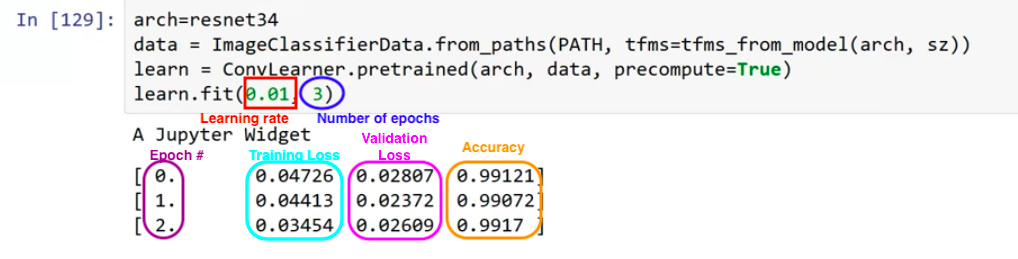
(5:00) The above sample code adjusts the Learning Rate, an adjustment to how fast the neural network adjusts weights. Setting a good rate will be the bulk of this lecture. Each Epoch is a pass through the data, running many mini-batches each updating weights, and then calculating the loss and accuracy of the new weights against the validation set. The Loss averages the ‘badness’ of each guess: “very sure its a cat” would give a loss near one if the image were a dog. The Accuracy is a simple ratio of the correctly guessed classifications over the number of samples, where the guessed classification is whichever one the model thinks is most likely, regardless of certainty. (1:12:00) You might also use a Confusion Matrix image to show true versus predicted labels.
Learning Rate
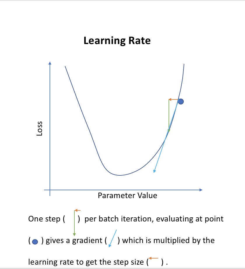
(4:50) The learning rate is an adjustment of how fast the neural network adjusts weights during training, or fast you try to hone in a solution. It is a Hyperparameter, meaning a tunable parameter of your machine learning engine. The FastAi Library picks reasonable values for dozens of hyper-parameters and reasonable choices for algorithms. You will learn when to override defaults throughout the course, and the library provides an estimator rather than a specific value for the learning rate. The learning rate is the most important hyperparameter.
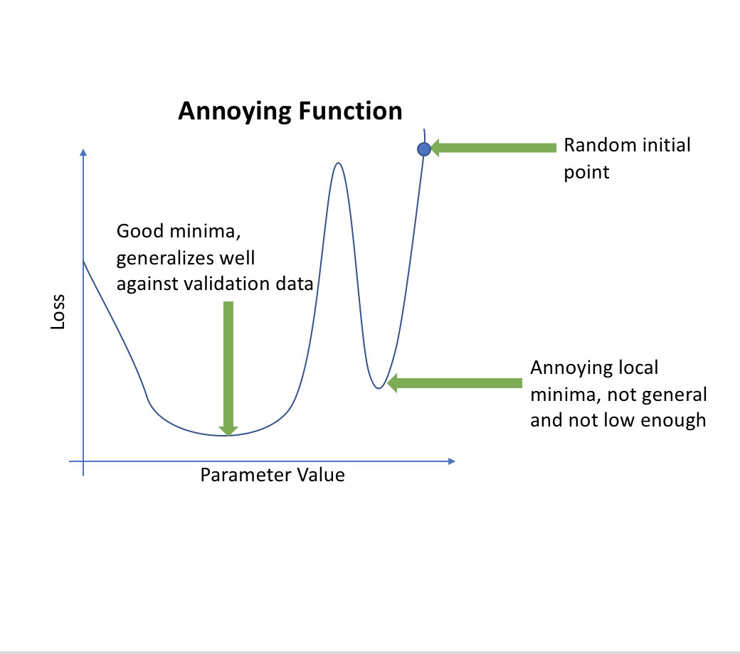
You can think of learning rate as length of the vector used in a step of gradient descent. If it is too low, the model will take too long to find the minimum and may get ‘stuck’ in a small local minima. If it is too high, it will jump around and follow a gradient to its nadir (lowest point). If you ever find your loss values going to infinity, your learning rate is too high.
There are three major methods presented: an algorithm for finding a good constant learning rate, simple Learning Rate Annealing where you decrease the learning rate as you train, and annealing with restarts where the learning rate decreases but gets reset after some number of epochs. There are also Differential Learning Rates which apply different rates to different layers of the model. All of these start by finding a good constant learning rate.
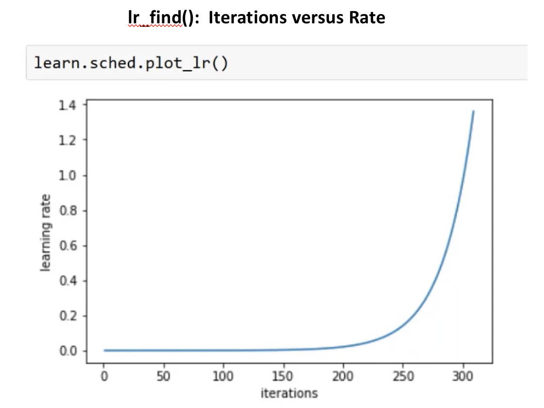
Constant Learning Rate with lr_find()
(7:30) The FastAI Library provides a Learning Rate Finder, or learn.lr_find():
- starting in random place with a small learning rate.
- on each minibatch, run a step, calculate the loss, and then multiplicitively increase the learning rate
- ignore the
learn.lr_find()output; look atlearn.sched.plot_lr()andlearn.sched.plot(). - best learning rate, is one order (10x) less than rate with minimum loss. In this case, 10e-2 (=0.01)
Three visualizations of this algorithm while finding the same learning rate:


Learning Rate Annealing and SGDR
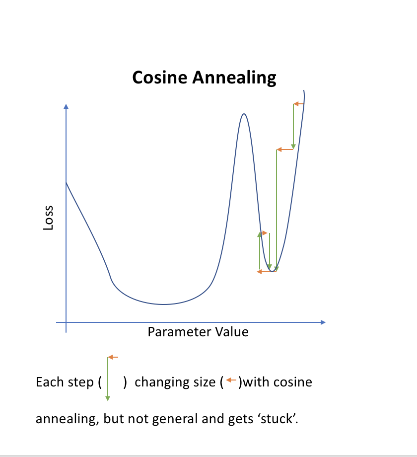
(34:00) Learning Rate Annealing is decreasing the learning rate as you train, hoping to find the nadir of the cost vs iteration function. It is a very common and popular technique. Three simple annealing methods start the learning rate at a constant (as found above) and gradually decrease the learning rate each mini-batch: Step-wise Annealing uses discrete decreases, sometimes in a manual or hacky way; Linear Annealing decreases learning rate a set amount per iteration; and Cosine Annealing uses the cosine curve from 0 to 90 degrees to reduce slowly then quickly then slowly again. A more complicated method would good results is Stochastic Gradient Decent With Restarts (SGDR) which periodically resets a simple (usually cosine) linear annealing curve every one or more epochs. This hopes to settle in “broad valleys” corresponding to good solutions that aren’t too specific to the specific training images. Use FastAI Library’s SGDR by adding the cycle_len=1 parameter to learn.fit(). (53:00) A final tweak on SGDR is to add the cycle_mult=2 parameter to continually increase the number of epochs between restarting the linear annealing curve.
These advanced SGDR routines work better than the approaches of a Grid Search (systematic search for good hyperparameter values) for a learning rate or Ensemble (run multiple models and take best result) of different starting points.
Compare the different learning rates over time with different methods.

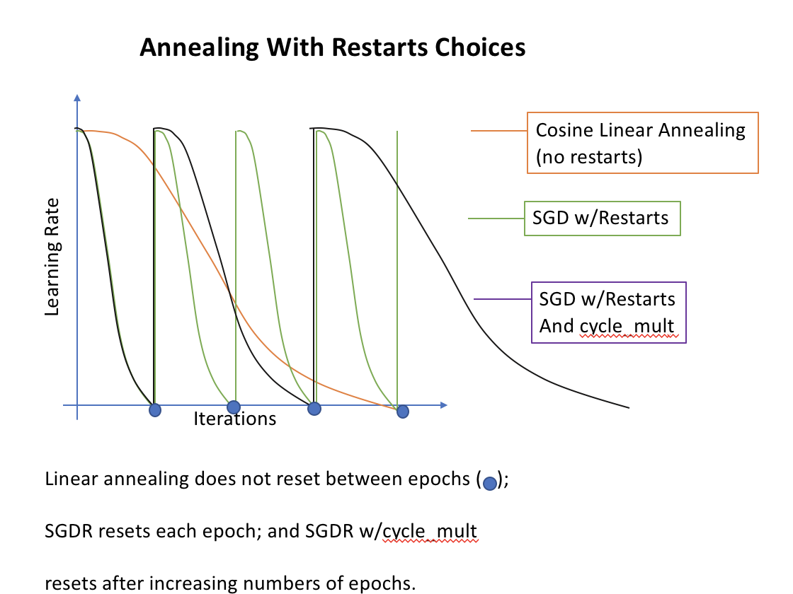
Consider how SGDR finds the general area of an annoying curve but simple annealing does not.

(46:30) After unfreezing the Early, Middle, and Later layers, we allow our training data to
adjust the weights of these layers, see About the Model. You can use Differential Learning Rates where different layers of the neural network have different training rates to tune the early layers less than middle layers less than later layers. To do this fine-tuning, use learn.unfreeze() then pass it to learn.fit(). (1:15:45) Usually use ratios of about 10x for regular images or 3x for medical or satellite images.
Data Augmentation
(15:00) Getting enough labeled data is always a problem. Without enough data, you get Overfitting where the network too closely memorizes artifacts of input data at expense of the actual meaning. Overfitting manifests as much lower training loss (more confidence) on your training set than your validation set and decreasing accuracy at later epochs. Getting more data is one solution.
Data Augmentation is creating additional synthetic data from existing labelled such that the bits change but not the meaning. This is done with transformation functions, e.g., “make new images by rotating the original image randomly between -5 degrees and +5 degrees”. The bits in each transformed image will be unique but the it will still be a cat. A typical set of transformations may include shifting, zooming, flipping, small rotations, or small brightness changes. A human chooses the set of augmentations that preserve meaning: faces flipped upside down are no longer normal faces. The FastAI Library lets you create a set of transforms (tfms_from_model) and pass them to the image classifier. At each minibatch during training, originals and random transformations will be used to train the model. (1:01:40) Padding and fixed sliding windows don’t work well and good transformations for non-image worlds are under-researched.
(54:30) You can also use Test Time Augmentation, which uses data augmentation at the testing time. Instead of classifying the validation image, classify the validation image and four random transformations of it and then take the average.
About the Model
Activation of any one node in the network is a number corresponding with how much one set of inputs match what the node was trained towards. (44:00) (1:45:00) A model can be thought of as Early Layers, Middle Layers, Later Layers, and a Final Layer. The ResNet model we use is based on a network already trained (weighted and biased) on all images of ImageNet. The Early Layers activate strongly to gradients and edges; the Middle Layers activate strongly to corners, circles and loops; and Later layers activate strongly to eyes, pointed ears, centers of flowers, faces, etc. In the original ResNet, the Final Layer connected to end of the Later layers and classified into hundreds of labels. (1:39:40) For our Cats and Dogs Model, the Final Layer was replaced with two layers to classify only Dog and Cat labels.
We are usually training only the final layer. The other layers (early, middle, and later) are Frozen, fixed such that training data will not affect their values. For efficiency, we use Precomputed Activations where we cache the activation values of the last of the Later Layers for each training image instead of recalculating each image each time it is in a minibatch, for about a 10x speedup. (41:00) We use precomputed activations with
ConvLearner.pretrained(arch, data, precompute=True) and these are stored in a dogscats/tmp directory. The first execution on a new dataset takes extra time to build the cache, except for Crestle which takes extra time more often. If everything hangs, try deleting the dogscats/tmp directory to reset the caches.
We need to turn off precomputed activations (learn.precompute = False) to use Data Augmentation. We unfreeze (turn off frozen) to use Differential Learning Rates.
About the FastAI Library
(1:05:30) The FastAI Library is open source on top of PyTorch, which is this year’s hot library. The FastAI Library makes PyTorch easier, but the concepts are the important part. In production, you might export the PyTorch models or recode in TensorFlow for use on phones.
Kaggle Competition
(1:13:52) To summarize the first hour, there is a sequence that usually can create a really good model. Roughly, its find the learning rate, train the last layer for couple epochs, train again with data augmentation, then differential learning rates, find the learning rate again, and finally train with SGDR w/cycle_mult.
(1:17:00) We will do this for the Kaggle competition on identifying breeds of dogs. We download the data with Kaggle CLI, get it loaded, and (1:23:30) explore the image sizes in
the sample. (1:26:40) We choose 20% to be the validation set.
While we first check our model with tiny images, we train with reasonable size. (1:33:00) After initial
training, we increase our image size to prevent overfitting.
We get a pretty good result without too much work. (1:53:00) We can also do this on the Planets competition.
(1:48:25) FYI, do even better on DogsCats using ResNext model instead!
While no homework is listed, there are a number of Kaggle competitions to try.
Shameless Plug: I’m leaving PARC at the end of January, 2018 and am looking for a fun start-up in Silicon Valley. charles.merriam@gmail.com
31 Likes
@CharlesMerriam that’s great! Would you be interested in contributing to our documentation project (with full credit of course)? It uses markdown, so we could potentially use your notes with just some minimal editing… 
Absolutely! I’ll also post the full sized slides (ppt) when I’m back at the right machine on Monday.
Let me know if you need any other action on my part; this parsed as just asking my permission.
No action required on your part - but more an optional thing that if you feel like there’s any edits you’d want to make to make your notes more widely useful, please do!
Done.
Hi everyone. I have done a quick proof reading and fixed, cleanup, corrected typos, reformatted style, etc. to ALL the lesson/lecture notes for version 2018 (aka part 1 v2) of this course. I hope the lecture notes are more pleasure to read now with those fixes in.
7 Likes
My hero! 
4 Likes
it provides better learning experience
I have been trying to understand this for a few time. I have watched lesson 2 in this regard.
Why is there the need for
precompute=True
in the above step for data augmentation step 4.
Please correct me if I am wrong. What I understand is: precompute is helping us getting the output(of the initial pretrained layers) for the same input again as no changes in all epochs. If we see an image we compute its output, save it, we see it again so we retreive that value as those initial layers are freezed so no need to compute again.
As we did data augmentation in the beginning so we already have all the data set with all the transformations. So when we did the step 3 of training the last layer we already have the values stored(for all the images including original as well as augmented ones), so why do precompute=False when using cycle_len=1 in step 4. And how can we say we are using data augmentation specifically in this case as the dataset is same since we have applied the transformations. If we set precompute to True in step 4 can’t we increase the efficiency?
2 Likes
Great work @timlee.
I noticed a typo here:
learn.set_data(get_data(299,bs))
learn.fit(1e-2,3,cycle_len=1)
learn.fit(1e-2,3 cycle_len=1, cycle_mult=2)
There should be a comma “,” on the last line after the “3” and before “cycle_len=1”
Thank you.
Lou
1 Like
in the get_data function , why are we resizing the using data.resize(340 , ‘tmp’) , instead it should be resized to using following : data.resize(sz , 'tmp)
Also why are we passing sz argument in tfms_from_model function.
Hi Cedric, Can you share a link to these notes? Thanks.
Hi, I should have been clearer. When I say “the lesson/lecture notes”, I meant to refer to timlee’s notes which is already in this forum in the form of wiki threads. An example of these notes:
Understood, thanks for the clarification.
Here is how my learning rate curve is looking. I’m not sure why. It doesn’t look anything close to what we see in cats vs dogs curve.
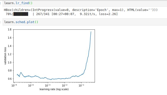
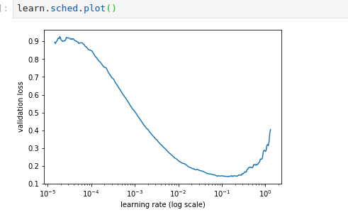
Just for the reference cats and dog’s learning rate curve looks like the one below.
Clearly something is wrong with the plot I’m getting for my dog-breed identification.
Can anyone please let me know about the learning rate curve they are getting?
Okie I tried few more things. here is what I found.
In the example code “learn = ConvLearner.pretrained(arch,data, precompute=False, ps=0.5)”
Notice the additional ps=0.5. With that Y-axis starts at 1.8 which is higher compared to 0.9 in the case of cats vs dogs lr_find().

Which results in the graph as below.
I removed that ps=0.5 value and now I’m getting the graph as shown below.
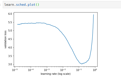
But now the Y axis is in the range 3 to 6. Looked in to the documentation for the class ConvnetBuilder
ps (float or array of float): dropout parameters
Not sure what droput parameter is at this moment. May be I’ll get to know in future lessons.