Another treat! Early access to Intro To Machine Learning videos

[radek]

Remember we’re limited to log2(n) binary splits per full decision, so we don’t want to waste any!

Is it a true statement: with enough data, I could do splits in any order and the trees will be equally good?

Every explanation of trees ever begins with addressing the best way to split because:
In reality, data log2(amount of data) doesn’t grow fast enough with the amount of possible split orderings, even with only 20 binary features we get 20! possible split orderings which is 2432902008176640000!

For comparison, with 100k examples we only get 16 splits!

It’s basically paper folding to the moon but in the other direction?

[radek]

BTW I have been banging my head against this whenever I ran into trees which I have done numerous times. I have never seen this addressed. Either I completely miss something here and what I write above completely doesn’t make sense, or the log2(n) insight was the piece I was missing.

I even asked this question on stackexchange and on reddit but the answers never touched on the core of the issue which I now am starting to see is the log2(n) thing - whether the tree would overfit or not if we go full depth (assuming full depth is possible) is IMHO completely secondary to figuring this out.

[Ekami (Tuatini GODARD)]

@jeremy a little question regarding the machine learning lesson 3 video at 47:20 where you say that: “Given the test set results from Kaggle and the results we have from our validation sets. We would like these 2 sets scores to be as linear as possible so that we know our validation set reflects the results we might have from the public leaderboard on Kaggle”.
So my question is: By doing so wouldn’t we be indirectly overfitting the public leaderboard? In other words: If we have a validation set which is pretty much the same as the Kaggle public leaderboard, how can we be sure that we are not tweaking our models to be good only at the public part of the leaderboard?
Thanks

[radek]

In proc_df:

def proc_df(df, y_fld, skip_flds=None, do_scale=False, na_dict=None,
            preproc_fn=None, max_n_cat=None, subset=None):
    if not skip_flds: skip_flds=[]
    if subset: df = get_sample(df,subset)
    df = df.copy()
    (...)

what does the last copied line do? df = df.copy()? Is there something on the df that copy discards that we want to get rid of?

[sermakarevich (sergii makarevych)]

df = df.copy()

I think it prevents modifying global df by making a local copy of it.

[Ekami (Tuatini GODARD)]

In python objects are passed as assignment which mean that: If we modify df directly we would modify the df object that was passed in by the caller. df.copy() means: "Duplicate this object so that next time lets say, I do df.dropna(inplace=True), the na will be dropped for the copy of df but not for the df that was passed in to proc_df"

[Ekami (Tuatini GODARD)]

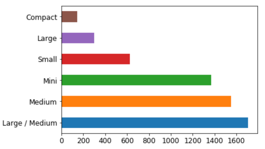
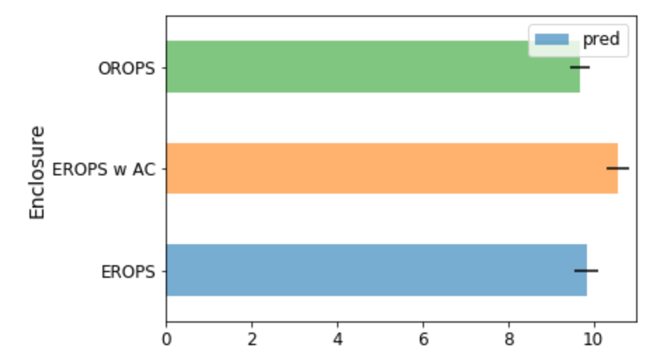
I didn’t quite understand what these confidence interval from lesson 3 were about. What exactly are we looking for with this? What am I supposed to understand or to “catch” when I look at those two graphs?

Thanks

[sermakarevich (sergii makarevych)]

There is nothing on the first chart as there are no confidence intervals. These small horizontal lines at the end of each bar show possible distribution of predicted values by different trees. If the line is short - you have good confidence in predicted value. If the line is long its like alarm alarm you have poor predictions for this category.

[Ekami (Tuatini GODARD)]

I still don’t get it sorry. At which point do we consider this line to be “wide”? And lets consider it is effectively wide on say, OROPS, what can we do about it? Should we just throw away this category?

[sermakarevich (sergii makarevych)]

As I understood these confidence intervals serve well for business insights. Bar on the chart is average of predictions from multiple trees. Sometimes these predictions are lower, sometimes they are higher than average. Confidence interval shows how much your estimation might vary for different trees. In credit score example bank might decide to not allow credit if credit score of a client is positive but confidence interval shows for some % of cases it can be negative.
For modelling purposes it might show categories where your predictions vary significantly. Significantly for me means higher % of variation compared to average per this category to variation of predictions for other categories.

[radek]

Are random forests just a way of partitioning very high dimensional space? All that happens is we pick some value from one of the dimensions and cut the entire space in half, coloring it with the mean of one group and the other half with the mean of the other group? And then we go on splitting to refine the partitioning?

That’s what a single tree would do - a forest just combines the colorings from each tree (space of whatever number dimensions) in some way, possibly via taking the mean?

Is there really all there is to this or could I completely be missing something?

[radek]

The curse of dimensionality

(Just to clarify: this discussion is about the machine learning course. In the future, we should try to keep these as replies in the machine learning discussion thread.)

The curse of dimensionality isn’t meaningful in practice because out space isn’t just a bunch of meaningless cartesian coordinates. We create structure, using trees, neural nets, etc. We regularize using bagging, weight decay, dropout, etc. We find that therefore we actually can add lots of columns without seeing problems in practice.

Accidentally discovered how to quote from other threads so moving the discussion over to here

I only finished watching lesson 2 but I think what @Ekami wanted to know - what are the reasons we remove some of the columns / data in lesson 3? As it is not because we inherently have something against having that many dimensions, why do we do it?

[radek]

In proc_df signature we set multiple default values to None

def proc_df(df, y_fld, skip_flds=None, do_scale=False, na_dict=None,
            preproc_fn=None, max_n_cat=None, subset=None):

and subsequently we mutate them if they are not set:

if na_dict is None: na_dict = {}

Is there a particular reason for this? It might be for nicer function signature but wondering if there is any Python related reason for this that I am not aware of?

[Ekami (Tuatini GODARD)]

In that case I also move my question here for which I didn’t find an answer in lesson 3:

Merging data from multiples datasets

I’m participating to the Favorita grocery Kaggle competition and my first approach to this challenge was to start by merging the different datasets between them as you can see on my kernel.
This would result in a train dataset of size 12gb compared to the original training data which size is 5gb.
Ofc I don’t plan to work on the entire dataset at first and I plan to use new Tensorflow Dataset API to read the resulting train/test csv iteratively.
But my questions are:

• Is it a good practice to start off by merging the tables when you start a new Kaggle competition? Then later on you do some feature engineering to transform/add/remove some features on your “big” dataset?
• Is there a much better way to merge/join the tables together than using pandas or sqlite? (for me I hesitated between using pandas and the .merge function as on my notebook and putting all the data in sqlite to join them using SQL. Because as you can see the csv files looks like they have been extracted from relational databases)

Thanks a lot for your help

This is more or less related to what we discussed about the curse of dimensionality earlier. Do we really want to merge this meta data to the rest of the training/test sets from the start?

[Ekami (Tuatini GODARD)]

I’m not sure about what I’m going to say but in the RL example @jeremy showed I think RF just stopped splitting its leafs at some point (based on the default hyperparameter max_depth I think) but these splits included data that were not really predictive. By removing them we allowed our trees to find the most relevant informations sooner and then ended up with trees of the same depth which splits were more “relevant”.

I think we could achieve the same level of “accuracy” with not removing the data but instead increasing the max_depth of the trees so they would split to something as relevant as if they directly started with the most important features.

Don’t hesitate to correct me on these statements, they are very speculative and can be completely wrong!

[radek]

All I do here at this point is also only speculation I think you are right - with infinite number of splits and compute this wouldn’t matter, but as we only have log2(n) of splits available, then for the 20k rows we use that gives us only 14 splits! Crazy when you look at the actual numbers involving logs / exps If we only have 14 splits, we want to use them as best as we can!

I am also thinking that that removal of data would not be necessary if we could have an arbitrarily large number of trees to fit. Then the noise would just cancel out I guess (assuming it was not super weirdly distributed?!). But since we can only have some probably small percentage of trees out of all the possibilities, we once again want to look at the relevant data - so we use what we learned earlier to limit the amount of garbage our model eats and feed it only the good stuff.

Only speculation so please take it with a grain of salt!

[jeremy (Jeremy Howard)]

Is it a true statement: with enough data, I could do splits in any order and the trees will be equally good?

That sounds right to me.

[jeremy (Jeremy Howard)]

By doing so wouldn’t we be indirectly overfitting the public leaderboard?

I addressed this in detail in today’s class - check for a new video tomorrow

[jeremy (Jeremy Howard)]

I think it prevents modifying global df by making a local copy of it.

Also, pandas normally returns a view into the original data, rather than actually changing the data. This can be slow and memory intensive.

[jeremy (Jeremy Howard)]

Are random forests just a way of partitioning very high dimensional space?

Yes exactly. Check out the proximity matrix for a really cool interpretation of this: https://www.stat.berkeley.edu/~breiman/RandomForests/cc_home.htm#prox